An Introduction to Information Infrastructure II
Editors: Alexander L. Hayes, Erika Lee, Shabnam Kavousian, Matt Hottell
An introduction to the infrastructure that runs our modern digital world. We introduce the technical background for informatics and computer science. This includes workflows and tools to help you be successful across a variety of computing disciplines. We will briefly review some math foundations, and then introduce programming languages, such as using Python for building backend systems. The final project is to build and deploy a full-stack web application.
We value computing as a discipline for everyone. We therefore aim to avoid misconceptions around computing and strive to keep the material as accessible as possible—accessible in terms of content (we will avoid hand-waving away the details as much as possible), and accessible in terms of monetary cost (this book is free to use, available under the terms of a fairly permissive creative commons license, and one of our goals is to eventually make it possible to be successful with this book without even owning a computer).
I211 Summer 2024
Hi friends! 👋
The key components of this class are the (1) lessons, (2) practice sets, and (3) the final project. This course is online and asynchronous, but we will stick fairly close with the schedule illustrated in this diagram:


How to succeed with technology
Imagine this situation: “You want an app that sends 30-second song snippets to your friends”.
Let’s imagine you have ten friends in this scenario. Would you rather: (Case 1) buy ten computers and mash buttons until all ten computers have an app that sends and receives song snippets? Or would you rather: (Case 2) write one program, and tell your friends to download an app?
Think about these cases for more than three seconds, you will likely conclude that case (1) would be extremely inconvenient for everyone. Buying ten computers would be expensive…. Writing custom programs for all ten computers would be time-consuming…. Delivering a computer to each friend would require coordination. Maybe you’re even a forward-thinking individual and realize that if something goes wrong (and our friend Murphy promises that something will go wrong) it could spell disaster. In the best case: there’s a problem on one computer, and your friend can send it back to you for repair; in the worst case you have to start this whole process from scratch. Buying new computers… writing new programs for them… delivering the new computers….
Why are we beleaguering this point? Well, we have some bad news. If you previously learned programming (either through being self-taught, learned during a course, or perhaps picked up from some basics introduced during high school) there’s a good chance that you were taught how to build hardware–not software.
The whole point of software, or “the code we write” is meant to contrast the hardware: or the physical infrastructure responsible for running the code we write. Hardware is typically whatever part is difficult, time-consuming, or expensive to change. Software–by contrast–should be anything that is easy to start and easy to fix. Therefore we’ll adopt a kind of five-point scale for everything we do:
| F | It doesn’t work | ⭐ |
| D | It sort of works on my machine | ⭐⭐ |
| C | It works on my machine | ⭐⭐⭐ |
| B | It sort of works | ⭐⭐⭐⭐ |
| A | It works | ⭐⭐⭐⭐⭐ |
“It works on my machine” is a meme in programming circles. It’s in the middle of our scale because it’s better than nothing: but we should be aiming higher. We’ll only consider things “to work” when we have a safe way to build, test, reproduce, and ship code to the end user. How do we do that? Read onward.
Python Cheat Sheet
Python is a strongly-typed, dynamically typed, interpreted, general-purpose programming language. The language is widely used for teaching, for data science or analytics, web development, or scripting.
This cheat sheet reviews core programming language concepts and vocabulary. This should get you back up to speed if it’s been a while since you’ve written in Python, or if you’re familiar with another language and need a rapid succession of examples.
Designing Programs
Programming language are built from five essential components.1
| Variables | store a value for later use. x = 1 |
| Conditionals | choose a behavior based on an observation. if, elif, else |
| Repetition | repeat a procedure until some condition is met. for, while |
| Abstraction | encapsulate a behavior; hide the details. def, class, import |
| Application | invoke an abstraction to return a result. x + 1 |
Every complex program—operating systems, video games, machine learning models, space shuttles—is at some low level of abstraction doing all five of these things. Major innovations happened over the last fifty years that made computers faster, smaller, and more affordable; but the core operation of transforming data is still here.
In “How to Design Programs”, Felleisen et al. define a “systematic program design” approach as the following six steps. When you’re working alone, these can guide you toward a solution. When you’re working with other agents—prompting large language models (LLMs) or asking someone for guidance—these can communicate where your thoughts are and how you organize ideas.
The Function Design Recipe
The “How to Design Programs” systematic design steps:2
- From Problem Analysis to Data Definitions. Identify the information that must be represented and how it is represented in the chosen programming language. Formulate data definitions and illustrate them with examples.
- Signature, Purpose Statement, Header. State what kind of data the desired function consumes and produces. Formulate a concise answer to the question what the function computes. Define a stub that lives up to the signature.
- Functional Examples. Work through examples that illustrate the function’s purpose.
- Function Template Translate the data definitions into an outline of the function.
- Function Definition. Fill in the gaps in the function template. Exploit the purpose statement and the examples.
- Testing. Articulate the examples as tests and ensure the function passes all. Doing so discovers mistakes. Tests also supplement examples in that they help others read and understand the definition when the need arises—and it will arise for any serious problems.
Starting and Stopping Python
In a terminal, we can start a Python REPL by running python3:
python3
The version numbers, dates, and platform information will look slightly different on different machines. But in general: the universal sign of a Python REPL is the triple greater-than signs: >>>
$ python3
Python 3.10.12 (main, Nov 20 2023, 15:14:05) [GCC 11.4.0] on linux
Type "help", "copyright", "credits" or "license" for more information.
>>>
REPL is an acronym for “Read-Eval-Print-Loop.” A REPL can be a helpful location for testing out our ideas, because its four steps give us instant feeback on everything we do:
- Read: Read an input expression from the user
- Eval: Evaluate the expression
- Print: Print the result of evaluating the expression, or show nothing
- Loop: Jump to (1)
When one is finished, calling exit() will quit out of the Python REPL, returning one back to their shell.
$ python3
>>> exit()
$
Primitive Types
A types or data type is a noun: they are the things or objects that we talk about in a language. A primitive type is the lowest level in a type hierarchy: they cannot be broken down into smaller units.3
| Type | |
|---|---|
int | -10 5 0 300 |
float | 0.1 0.2 -10.5 1e5 1e-3 |
bool | True False |
str | "0" "5" "xyz" 'hello' |
None | None |
There is another word you may encounter at this level: the object. We will use the words type and object interchangeably. This is because defining a new object is really defining a new type of data: a data modeling problem.
Type Casting
Type casting happens when we convert something from one type to another.
Sometimes this change is lossless when there is a one-to-one relationship between the data types:
>>> int(False)
0
>>> int(True)
1
>>> int("123")
123
>>> str(123)
'123'
Other times changing the data type is lossy. Information about the underlying data is lost when we convert from one representation to another:
>>> int(2.5)
2
>>> float(2)
2.0
>>> float(int(2.5)) == 2.5
False

>>> float(str(2.5)) == 2.5
True
Truthiness
Truthiness is the idea that some types are inherently True and others are inherently False. A type’s truth can be checked by casting it to a bool:
>>> bool(0)
False
>>> bool(1)
True
As a rule: Falsey values correspond with emptiness, nothingness, or zero-ness.
>>> bool(0)
False
>>> bool(None)
False
>>> bool("")        # the empty string is `False`
False
>>> bool([])        # the empty list is `False`
False
Everything which is not False is True. Truthy values therefore correspond with full-ness, something-ness, or existence. For example, every non-zero number is True:
>>> [i for i in range(-3, 3)]
[  -3,   -2,   -1,     0,    1,    2]

>>> [bool(i) for i in range(-3, 3)]
[True, True, True, False, True, True]
Identifiers, Variables, and Names
A variable binds an identifier to a value through assignment with the equal sign =:
>>> x = 1
>>> x
1
Variables vary in that re-assigning an identifier to a new value changes its value:
>>> x = 1       # assign `x` to `1`
>>> x = 2       # re-assign `x` to contain `2`
>>> x
2
An identifier is a letter-number combination:
>>> x1 = -1
>>> x2 = "a"
Identifiers must start with a letter, and there exist many symbols which the language does not consider as valid parts of an identifier.
>>> 📦 = 1          # SyntaxError
>>> $ = 1           # SyntaxError
>>> 1c = 1          # SyntaxError: starts with a number
>>> one! = 1        # SyntaxError
Some identifiers are reserved by the language. This barrier prevents potentially dangerous side effects, like changing the meanings of True and False.
The full list of Python’s reserved keywords are maintained in Python’s lexical analysis documentation.
False      await      else       import     pass
None       break      except     in         raise
True       class      finally    is         return
and        continue   for        lambda     try
as         def        from       nonlocal   while
assert     del        global     not        with
async      elif       if         or         yield
Finally, a defined identifier is given a special title, a name. Trying to invoke a name that does not exist is therefore a NameError:
>>> v
NameError: name 'v' is not defined
Expressions, Math, and Operators
Wikipedia phrases an expression as “A syntactic entity in a programming language that may be evaluated to determine its value.”4 Translating from Wikipediese, we have two things: a syntactic entity, and evaluation. A syntactic entity for our purposes means “a valid piece of Python code”.
The simplest expressions are the primitive types, and the simplest rule of evaluation is that every primitive type evaluates to itself:
>>> 0
0
>>> 1
1
>>> 'foo'
'foo'
>>> True
True
>>> None
None
More interesting expressions involve combining primitive types with operators and operands. By example: in the expression 0 + 4, the plus + symbol is an operator, while 0 and 4 are the operands in the expression.
>>> 0 + 4
4
>>> 0 - 4
-4
In concert, operators and operands answer the question: what action is being carried out, and what is it being carried out upon?
Understanding evaluation in full quickly devolves into trying to comprehend “how does Python actually work?” So the simple definition that we will stick with is that “evaluation is the 2nd step in REPL, where a piece of code turns into a result”.
Since operators (+, -) act upon types/objects/operands, we’ll extend our analogy to say that types are to nouns as operators are verbs.
$$ \text{type} : \text{noun} :: \text{operator} : \text{verb} $$
This gives us the logical operators, math operators, and binary relations:
| Symbol | Operator Name | Usage |
|---|---|---|
+ | addition | (2 + 5) == 7 |
- | subtraction | (5 - 2) == 3 |
* | multiplication | (5 * 7) == 35 |
// | floor division | (36 // 7) == 5 |
% | modulo (remainder) | (10 % 9) == 1 |
** | exponentiation | (2 ** 3) == 8 |
/ | (float) division | (6 / 4) == 1.5 |
and | logical and | True and True |
or | logical or | True or False |
== | equal | 1 == 1 |
< | less than | 2 < 3 |
> | greater than | 3 > 2 |
<= | less than or equal | 2 <= 3 |
>= | greater than or equal | 3 >= 3 |
!= | not equal | 2 != 3 |
Expressions themselves may contain other expressions. Evaluation must therefore act on tree structures, which for math operators follows the PEMDAS rules (parentheses, exponentiation, multiplication, division, addition, subtraction). Or one may be precise and add parentheses to specify a particular order:
>>> (0 + 4) + (0 - 4)
0
graph TD
    A["+"]
    A-->B["+"]
    B-->C[0]
    B-->D[4]
    A-->E["-"]
    E-->F[0]
    E-->G[4]
versus the case without parentheses:
>>> 0 + 4 + 0 - 4
0
graph TD
    A["+"]
    A-->B[0]
    A-->C[4]
    D["+"]
    D-->A
    D-->E[0]
    F["-"]
    F-->D
    F-->G[4]
Finally, evaluation is done with respect to an environment. In this context,5 an environment is the set of all valid names when evaluation happens. Therefore an environment is a kind of mapping between identifiers and their value, allowing us to express ideas which require storing data and retrieving it later.
>>> ZERO = 0
>>> ONE = 1
>>> ZERO + ONE
1
graph TD
    subgraph environment
    ZERO-->0
    ONE-->1
    end

    subgraph evaluate
    A["+"]
    A-->B[ZERO]
    A-->C[ONE]
    end
From Operators to Functions
Operators and operands are implemented in Python using functions. So what is the difference between an operator and a function? In theory: nothing. In Python: how we use them. Peruse your keyboard, is there a symbol on it that represents the concept of maximum or minimum? There isn’t an agreed-upon standard, so the symbol for maximum is usually the word max.
>>> max(1, 3, 5, 2, 4, 7, 6)
7
>>> min(1, 3, 5, 2, 4, 7, 6)
1
The Python language developers built common functions into the language for many of the routine operations that programmers need to accomplish. Types and control flow around types:
bool()dict()float()hex()int()len()list()set()str()tuple()type()isinstance()
Logic and math functions:
all()any()abs()hash()max()min()pow()round()sum()
Debugging and input/output control:
breakpoint()dir()format()help()id()input()open()print()
And finally, iteration controls and higher-order functions:
enumerate()filter()map()next()range()reversed()sorted()zip()
A function is a verb: and verbs accomplish goals. A function takes some arguments and returns some outcome.
$$ \text{type} : \text{noun} :: \text{function} : \text{verb} $$
In Python and most other programming languages, subject-verb phrases must be written so as to be explicit about which verbs act on which nouns. “Unload the couch from the truck” is valid English, but we must be precise and express that we have a truck (noun), and we receive the couch (noun) when we unload (verb) the truck.
couch = unload(truck)
Defining New Functions
A function is created through definition with the def statement, and every function will return something when it completes. Since functions must always be explicit about the objects they act upon: zero or more objects are passed into the function, and one or more value is returned at the end.
def _____():                    # 0x1
    return _____


def _____(_____):               # 1x1
    return _____


def _____(_____, _____):        # 2x1
    return _____


def _____(_____, _____):        # 2x2
    return _____, _____
Every function returns something. Functions that do not explicitly return something will return None:
>>> def does_nothing():
...     pass
...
>>> does_nothing()
None
Local and Global Scoping
Scoping rules govern the relationship between where a name gets defined and what that name means.
Names fall into one of two categories: local and global. For example, if we bind the value 1 to the name x in a global scope, then that variable will also be available from within a function:
x = 1

def returns_x():
    return x

print(returns_x())
# 1
But the inverse is not true. Functions are like Vegas: names defined in the function stay in the function.
def returns_1():
    v = 3
    return 1

print(v)
# NameError: 'v' is not defined
Scoping rules in Python obey a specific set of behaviors called lexical scoping or lexical addressing. In the formal study of programming languages, one would learn the relationship between the context in which a name is defined and the context in which that name is evaluated. Puzzles for a niche audience: why does the following print 1?
y = 3

def y(x):
    def y(x):
        y = 1
        return y
    return y(x)

print(y(3))
The strategy we will recommend is to minimize global state, and prefer any global behaviors are treated like immutable or constant data—data that are declared once and never modified. A convention is to declare these variables with “screaming snake case”: where all letters are capitalized and words are separated by underscores when necessary. For example, a program that uses a comma-separated value (CSV) file might declare a global set of strings representing column names. This global state can then be used to enforce consistency when reading, writing, and performing error handling:
import csv

EXPECT_COLUMNS = ["id", "name", "phone"]


def inspect_csv(file_name: str) -> bool:
    """Does the first line of a .csv file have the correct header?"""
    with open(file_name) as csvf:
        for first in csv.reader(csvf):
            return first == EXPECT_COLUMNS


def load_people(file_name: str) -> list | None:
    if not inspect_csv(file_name):
        return None

    with open(file_name) as csvf:
        return list(csv.DictReader(csvf))


if __name__ == "__main__":
    print(load_people("people3.csv"))
⚠️ Danger: Forcing Local or Global Behavior
Python reserves two keywords:
nonlocalandglobal, which allow programmers to switch between local and global contexts on demand.We mention this because you should avoid this. Consider the difference between this program, which should obviously raise a
NameErrorsincexis a local variable:def foo(y): x = y return y foo(3) print(x) # NameError: 'x' is undefined.Contrast it with this, which will print
3:def foo(y): global x x = y return y foo(3) # Calling `foo` changes the value of `x` print(x) # 3Left unchecked, this is a slippery beetle into bugs. Programs that use global mutable state, such as assigning to global variables, become difficult to reason about as they grow. Instead: keep most variables scoped inside of functions, and minimize how much global data there is.
Dynamic Typing and Function Polymorphism
Python is dynamically typed: meaning that every variable in the language has a type, but that type can change at runtime. This also means that Python functions behave differently according to the data that are passed into them. A function like:
def sum_three(x, y, z):
    return x + y + z
… should have an obvious interpretation when x, y, and z are integers:
>>> sum_three(1, 2, 3)
6
But this interpretation may be less obvious when x, y, and z are strings:
>>> sum_three("a", "b", "c")
'abc'
… or lists:
>>> sum_three([1], [2], [3])
[1, 2, 3]
This is called polymorphism: operations like plus + behave differently depending on the data type. When we have two variables \(x\) and \(y\), and we know they contain numbers \((x, y) \in \mathbb{Z}^{2}\) then we call the + operator “addition”. If instead \(x\) and \(y\) are strings, then we call the + operator “concatenation”.
A polymorphic function is therefore a function that behaves differently depending on what gets passed into it. Often this is advantageous, but may also be a source of unexpected bugs. How might be be explicit about the data types that we expect our functions to work with?
Functions with Type Annotations
When declaring a function, one may use the name of a variable, a colon :, and a type to declare the types of values that the function expects. This can make it more clear to ourselves, other programmers, or other entities how we expect parts of the program to behave.
def sum_three_nums(x: int, y: int, z: int) -> int:
    return x + y + z
def _____(_____: ___, ...) -> ___:
    return _____
Note that current versions of Python treat type annotations like guidelines. Other tools do exist to validate types through various approaches collectively called static analysis. One can declare and call functions that clearly violate the type signatures:
def bar(x: int) -> int:
    return x

print(bar("str, not int"))
But tools like mypy or Visual Studio Code’s Pylance language server’s typeCheckingMode treat type errors as actual errors:
$ mypy bad_typing.py
bad_typing.py:4: error: Argument 1 to "bar" has incompatible type "str"; expected "int"  [arg-type]
Found 1 error in 1 file (checked 1 source file)
Statements: Conjunction and Control Flow
So far we have types (nouns) and operators/functions (verbs), but the ideas we may express are limited without some way to link different clauses together.
Python, and many languages derived from C, follow a procedural programming view. In it: most core program behavior should be defined inside of types and functions that call and refer to each other, all mediated via control flow mechanisms. The English words if, for, and while connect clauses—but in Python these words affect our interpretation on how the types and functions relate to overall program behavior.6
$$ \begin{align} \text{type} &: \text{noun} \cr \text{function} &: \text{verb} \cr \text{statement} &: \text{conjunction} \end{align} $$
Python defines simple statements as any statement taking zero or one arguments:
| Statement | Example | Result |
|---|---|---|
return |
|
foo() == 1 |
del |
|
x == {} |
pass |
|
bar() == None |
continue |
|
total == 4 |
break |
|
total == 0 |
import |
|
(csv module available) |
Compound statements refer to everything else, and you can recognize one because they are always accompanied by a colon :.
defif,elif,elseforwhilewithtry,except,except*,else,finally
Data Structures and Collections
A data structure is a particular way to arrange a collection of objects such that efficient algorithms may be built on top of them. Algorithm design and analysis is an advanced topic in computer science that we will not cover. However: many smart people already did that work, and you can benefit from their knowledge.
The three fundamental data structures in Python are lists, tuples, and dictionaries. Many more exist, but the core language and all other data structures may be explained in terms of these three.
Lists are ordered sequences of items, represented with square brackets: [, ].
>>> lst1 = [0, 1, 2, 3, 4]
>>> lst2 = [4, 3, 2, 1, 0]
Dictionaries are unordered mappings that implement an association between a key and a value. These act like physical dictionaries where each word has a meaning: making each word a key and the meaning its value.
vocabulary = {
    "python": "a programming language",
    "list": "an ordered sequence",
    "dictionary": "an unordered mapping",
}
Tuples are ordered sequences of items. Unlike lists: they are immutable. Tuples are often mistaken as being represented by parentheses (, )—the reality is that the parentheses are convenient, but the comma , is all that one needs to represent a tuple:
red = 255, 0, 0
green = 0, 255, 0
blue = 0, 0, 255
Understanding these three data structures gives enough mental scaffolding to understand most other data structures. For example, a set is an unordered collection which can answer whether an element is a member of the set or not. In other words: a set is like a dictionary that only has keys.7
>>> some_set = {"Alexander", "Erika"}
>>> like_a_set = {
...     "Alexander": 0,
...     "Erika": 0,
... }
...
>>> some_set == like_a_set.keys()
True
Dictionaries
Recall that dictionaries are collections of key, value pairs. We’ll usually recommend keeping dictionary types simple: such as mapping from strings to integers dict[str, int], or strings to strings dict[str, str]. Also recall that dictionary keys must be unique and immutable (e.g. str, int, tuple), but their values can be any data type: including other lists or other dictionaries.
Dictionary values are accessed via their key:
>>> fruit = {"apple": 1, "orange": 3, "pear": 2}
>>> fruit["pear"]
2
Attempting to access a key that doesn’t exist in the dictionary is a KeyError:
>>> fruit = {"apple": 1, "orange": 3, "pear": 2}
>>> fruit["kiwi"]
Traceback (most recent call last):
  File "<stdin>", line 1, in <module>
KeyError: 'kiwi'
… unless one uses a dictionary’s .get method, which returns None to indicate absense, or returns a default value if one is provided:
>>> fruit = {"apple": 1, "orange": 3, "pear": 2}
>>> print(fruit.get("kiwi"))
None

>>> fruit.get("kiwi", 0)
0
Updating a (key, value) pair uses assignment = to assign a key to a new value:
>>> fruit = {"apple": 1, "orange": 3, "pear": 2}
>>> fruit["apple"] = 1000
>>> fruit
{'apple': 1000, 'orange': 3, 'pear': 2}
… or if one assigns a value to a key that does not exist, they will be added:
>>> fruit = {"apple": 1, "orange": 3, "pear": 2}
>>> fruit["tangerine"] = 75
{'apple': 1, 'orange': 3, 'pear': 2, 'tangerine': 75}
Removing something from a dictionary may be done using the del keyword:
>>> fruit = {"apple": 1, "orange": 3, "pear": 2}
>>> del fruit["orange"]
>>> fruit
{'apple': 1, 'pear': 2}
Nested and Composite Data Structures
Continuing the vocabulary analogy, the Merriam Webster English dictionary presents multiple word meanings.
mw = {
    "guardrail": [
        "a railing guarding usually against danger",
    ],
    "balustrade": [
        "a row of balusters topped by a rail",
        "a low parapet or barrier",
    ]
}
Indexing, Selecting, Slicing, and Attributes
Selecting data out of a data structure is one of the most routine operations used across programming. Selecting data requires some definition of an index to exist: where in the data structure is the information that one needs? The exact nature of how indexing works is a topic for another time, but the three most common flavors to be aware of are
- integer-based: used by lists
- key-based indexing: used in dictionaries
- attribute-based indexing: used in everything else
Lists are indexed using integers. A list has some fixed number of items in it, and each item therefore must have an ordered position in the list. If one has a list of tasks that they want to accomplish:
tasks = ["write", "edit", "get feedback"]
One can visually inspect the code to see that the list contains three things. Python’s syntax for selecting data out of a list involves square brackets [] and the index position of the item in the list:
>>> tasks[0]
'write'
>>> tasks[1]
'edit'
>>> tasks[2]
'get feedback'
Dictionaries behave similarly, but similar to how one would look up a word in a physical dictionary or online dictionary: each item in the dictionary is a \((key, value\)) pair, so one may look up the value by looking up the key. For example, if you choose to represent the workouts you do on each day of the week as a dictionary, the keys could be the name of each weekday and the values could be the associated exercise for that day:
workout_routine = {
    "Monday": "Cardio",
    "Tuesday": "Core",
    "Wednesday": "Rest",
    "Thursday": "Leg Day",
    "Friday": "Upper Body",
}
Selecting the weekday from the dictionary will therefore result in the value for what should be done on that day:
>>> workout_routine["Wednesday"]
'Rest'
>>> workout_routine["Thursday"]
'Leg Day'
Integer or key-based indexing is sufficient to extract one item at a time, but what if we need to handle multiple items at a time? Imagine we’ve been keeping track of our heart rate, but we want to know what the average heart rate is over some period of time. If we measure our heart rate every minute for five minutes, then we’ll have a list of five heart rates:
heart_rates = [74, 77, 78, 77, 75]
Slicing represents extracting consecutive elements in a list—as if you have a Nerds Rope in front of you and you want to split the candy into three pieces, then imagine you have a knife and make a few cuts:
heart_rates = [74,  77,  78,  77,   75]
              ---- --------------  ----
              [74] [77,  78,  77], [75]
One can slice from \((0, 1)\) to get a list containing the first item in the list, or slice from \((1, 4)\) to get the middle three elements, or slice from \((4, 5)\) to get a list representing the last thing in the list.
>>> heart_rates[0:1]
[74]
>>> heart_rates[1:4]
[77, 78, 77]
>>> heart_rates[4:5]
[75]
The underlying object that accomplishes this in Python is the slice object, requiring a start and an end (and optionally a step, representing a kind of skip or stride or every other element in the slice(None, None, 2) but for now understanding the start and end point in a list is more than sufficient).
Slicing can therefore be used as a way to represent concepts like the first two items:
>>> heart_rates[:2]
[74, 77]
… or the last two items:
>>> heart_rates[-2:]
[77, 75]
… or everything between the first and last element:
>>> heart_rates[1:-1]
[77, 78, 77]
To round this out: many data structures in Python are implemented in terms of objects, usually defined with a class. We mentioned earlier that we use the words type and object interchangeably. If we define a new type to represent some point in two-dimensional space:
class Point:
    def __init__(self, x, y):
        self.x, self.y = x, y
    def __repr__(self):
        return f"Point({self.x}, {self.y})"
… then we’ve defined a new noun in our language. From the __init__ definition (sometimes called a constructor or initializer), we can see that a Point has an x and y coordinate. The names x and y are available to anyone who uses this type, finally bringing us to attribute-based indexing. Attribute-based indexing looks similar to the key indexing we saw with dictionaries,8 but now the indexing is performed using a period or dot and the name of the attribute one intends to access.
For example, the origin in a coordinate system is \((0, 0)\). If we instantiate a variable named origin, then we may later access origin.x for the \(x\)-coordinate and origin.y for the \(y\)-coordinate:
>>> origin = Point(0, 0)
>>> origin.x
0
>>> origin.y
0
Even if you aren’t defining your own types, you might often be working with a type that is built into the language, and therefore may need to know how to look up the value of an attribute defined on that type. Remember those slices we just mentioned? The start and stop values are available as attributes after initializing a slice:
>>> slc = slice(0, 3)
>>> slc.start
0
>>> slc.stop
3
Or if you’re diving into how some of the built-in types actually work, you might find out that every integer also has some attributes defined on them: a numerator and denominator:
>>> x = 7
>>> x.numerator
7
>>> x.denominator
1
To review: indexing is how Python represents where something is, and indexing comes in three varieties (integers, keys, and attributes). The three approaches are mixed and matched in order to select data out of composite data structures by following the access logic. If one represents a triangle as a list of three points, then one may can access the \(x\)-coordinate of the first point with the integer [0], then with the attribute .x.
>>> triangle = [Point(0, 1), Point(3, 1), Point(5, 4)]
>>> triangle[0].x
0
>>> triangle[1].x
3
>>> triangle[2].x
5
Iterables and Ordering
Iteration is a single step in a sequence—progressing toward completion. One may iterate on their current draft in order to make it better. We already mentioned loops (while, for) and said that there were built-in Python functions related to iteration:
for i in range(3):
    print(i)
# 0
# 1
# 2
An iterable is therefore any type, data structure, or object which may be iterated with a loop. Many objects which can be thought of as an ordered collection of smaller objects—like strings, lists, or tuples—are also iterable. For example, we might iterate over a list of words (strings), then iterate over each letter in each word:
words = ["foo", "bar", "baz"]

for word in words:
    for letter in word:
        print(letter, end=" ")
# f o o b a r b a z
However, one should be mindful that there do exist things which are not ordered, but are iterable. We said earlier that sets and dictionaries are unordered collections of objects. Despite not having an obvious ordering, both data structures may be iterated over with a loop.
The important point to keep in mind is that the order that one may expect may not be the one that Python uses. In the workout dictionary, the English names “Monday” through “Friday” may have some semantic meaning when a person reads them:
workout_routine = {
    "Monday": "Cardio",
    "Tuesday": "Core",
    "Wednesday": "Rest",
    "Thursday": "Leg Day",
    "Friday": "Upper Body",
}
But will Python iterate through the keys in that order?
>>> for day in workout_routine:
...     print(day)
Monday
Tuesday
Wednesday
Thursday
Friday
In this case: yes 😉 Python 3.7 started enforcing that for objects which are otherwise considered to be “unordered”: the iteration order is the same as insertion order. Since workout_routine was initially defined with "Monday" at the beginning and "Friday" at the end: that order is invariant when we check the order later.
This means that if we wanted to write a program to assign a random exercise goal to each day of the week, we might preserve the weekday order by preserving the order of keys going into the dictionary:
from random import shuffle

weekdays = ["Monday", "Tuesday", "Wednesday", "Thursday", "Friday"]
workouts = ["Cardio", "Core", "Rest", "Leg Day", "Upper Body"]

shuffle(workouts)

this_week = dict(zip(weekdays, workouts))

for day, exercise in this_week.items():
    print(f"{day} -- {exercise}")
# Monday -- Leg Day     (random outputs)
# Tuesday -- Cardio
# Wednesday -- Core
# Thursday -- Rest
# Friday -- Upper Body
Functions as Tuples or Dictionaries
Knowing about tuples and dictionaries provides one more way to think about functions. So far we’ve treated functions as a name (like foo) accompanied by an ordered set of arguments.
def foo(x, y):
    return x + y
An ordered, immutable set of arguments is equivalent to how we defined tuples.
>>> args = (3, 5)
>>> foo(*args)
8
Similarly, keys and values are similar to how we thought about dictionaries. When defining functions, we can define keyword arguments which can take on default values when calling the function:
def bar(x, y, base=0):
    return x + y + base
or
def baz(x, y, debug=False):
    if debug:
        print(x, y)
    return x + y
Methods
Methods are special kinds of verbs: reflexive verbs. Reflexive verbs happen in English when an agent does something to itself. For example:
- One can “self-describe” - only you can self-describe you
- You can “self-evaluate” - but no person can self-evaluate you
- One can “perjure” - but one cannot perjure someone else
$$ \text{type} : \text{noun} :: \text{method} : \text{reflexive verb} $$
A method is a function defined on a type. We can access methods with dot notation: calling a method similar to type.method() causes something to happen.
Methods that take an argument often modify the underlying type in some way, such as appending something to a list.
>>> lst = []
>>> lst.append(3)     # "append 3 to yourself"
>>> lst
[3]
A method can also answer a question about the underlying data. What keys are in a dictionary? We can check by querying .keys():
>>> dct = {0: 1, 1: 2}
>>> dct.keys()
dict_keys([0, 1])
Modules
Names are also assigned on a per-module or per-file basis. If one has two Python scripts: printer.py and writer.py, then one cannot use a function from one without first importing it.
# writer.py
def make_title_case(title: str) -> str:
    """Convert a space-separated string to titlecase.

    Unlike `.title()`, this does not convert numbers to all-caps.
    """
    title_words = []
    for word in title.split():
        title_words.append(word[0].upper() + word[1:])
    return " ".join(title_words)
# printer.py
from writer import make_title_case

print(make_title_case("autobiography of mark twain"))
# Autobiography Of Mark Twain
Data Representation
Let’s wrap up this cheat sheet by talking about design choices. As programmers, software engineers, or developers—we’re often making decisions about how we write our code in order to best maintain the software over time, or to meet some external criteria (readability, scalability, testability, reliability, and a whole scrabble board of words ending in -ility). The code we write, and the data that the code operates on is therefore subject to decisions about how everything in our representation of the universe should work.
Let’s use color as an example.
Colors in HTML and CSS are red/green/blue RGB triples defined with three integers between 0-255. This true color, or 24-bit color depth, used on just about every mainstream computer display is capable of rendering 16,777,216 colors.
But let’s stick with five colors that we may believe are sufficient for a problem we’re working on. Should we store colors like this:
colors = {
    "white": "ffffff",
    "black": "000000",
    "red":   "ff0000",
    "green": "00ff00",
    "blue":  "0000ff",
}
or should we represent the colors like this?
colors = {
    "white": (255, 255, 255),
    "black": (0, 0, 0),
    "red": (255, 0, 0),
    "green": (0, 255, 0),
    "blue": (0, 0, 255),
}
One could say well it depends because it always does, but that advice is general to the point of being useless. A more interesting answer is that the two representations are actually the same. Representing "black" with the tuple (0, 0, 0) or the string "000000" are two representations of the same concept. (0, 0, 0) is more explicit about the view that true color is comprised from three components R/G/B. The hexadecimal number "000000" might be less transparent about this fact at first, but this representation could be ideal for readers who are (1) already aware of the hexadecimal representation, or (2) end users or downstream programs which will eventually need an HTML-like hexadecimal number anyway.
Here’s the advice: don’t overthink these decisions, but don’t underthink them either. Software is meant to be soft—one may only figure out much later which decision was ultimately correct. Should one be paralyzed by indecision trying to reason through all possible decisions and the downstream effects of all possible decisions? No! Time is better spent designing a prototype and iterating on it as new feedback and new information comes in.
Since this color example shows two equivalent representations, there’s another option: store the data in one way, but if you need the other representation at any point, one could convert between the two representations with a function:
def color_to_hex(r: int, g: int, b: int) -> str:
    return "".join((c).to_bytes(1, "big").hex() for c in (r, g, b))
One could even define a new data type representing the TrueColor, and define methods and properties on this type to build these behaviors into the representation:
class TrueColor:
    def __init__(self, r: int, g: int, b: int):
        self.r, self.g, self.b = r, g, b

    @property
    def hex(self) -> str:
        return "".join((c).to_bytes(1, "big").hex() for c in (self.r, self.g, self.b))

    def __repr__(self):
        return f"TrueColor({self.r}, {self.g}, {self.b})"
But here inlies the chief tension: building new levels of abstraction comes with an intellectual cost. When something needs to change in the future (and tech changes quickly: it will need to change in the future and the due dates may approach rapidly), one may need to traverse mountains of abstractions even to make what feel as if they should be simple changes.
So as parting advice: aim for a kind of minimalism in the code you write. Flexibility and the ease with which one can read, understand, and modify code should be its own reward.9
Footnotes
These five follow from a procedural approach to programming and programming languages. Other paradigms exist which may appear to bend these rules—such as structured query language (SQL), which is an instance of a declarative language. A lambda calculus approach to studying languages would tell you that all computation can actually be done with three rules: definition, abstraction, and application—the astute reader may wonder where concepts like conditions and repetition went? The answer is that those concepts can just as easily be defined in terms of abstraction and application.
From: Felleisen et al. 2014, “How to Design Programs”. Used under the terms of the Creative Commons CC BY-NC-ND license. Online: HTDP, Preface, Systematic Program Design
Lower levels do exist: in Python at least, every type has an associated class or metaclass. Furthermore, the float or int types in particular have binary representations, and at the lowest level: computers are moving bits around. Awareness of these details—that technically there is something lower than the primitive types—makes for a more accurate representation. But we can be productive without this detail, whereas digging into this footnote further would quickly lead us down the path of: “but how exactly does Python work?” Our goal is to eventually build web applications, a theoretical study of programming languages and how they actually work is outside our scope.
As we’ll see later when we talk about virtual environments, the word environment is overloaded in informatics, computing, and engineering. But even when the word is used differently, the texture is the same: an environment always represents a set of assumptions that get passed along with the code we write. The nature of the environment will grow more complex at higher levels of abstraction though: at a low level an environment represents all the valid variables, and at a high level the environment will refer to the state of entire computers or networks of computers working together.
But one may also ellide conjunctions altogether using functions by making more λs.
In fact, sets in Python originally were dictionaries. It’s wasteful to store values that aren’t needed though, so after a few releases the Python developers optimized away the extraneous values.
The similar appearance of key indexing (foo['x']) and attribute indexing (foo.x) has a deeper reasoning: every object in Python is implemented as what we call a “thin wrapper” around a dictionary. With a few steps, one could even define data structures that further blur the lines between objects and dictionaries by automatically making attributes available as keys and vice-versa (for example, see the scikit-learn Bunch object: https://scikit-learn.org/stable/modules/generated/sklearn.utils.Bunch.html)
Chris Hanson and Gerald Jay Sussman, “Software Design for Flexibility: How to Avoid Programming Yourself into a Corner”. The MIT Press, 2021-03-09, 978-0-26204549-0
I211 Debugging and Shortcuts
TL;DR Review Sheets
Many chapters end with a “Too Long; Didn’t Read” or “TL;DR” guide which should be reviewed frequently:
- Essential git terms and commands
- Daily VS Code and git/GitHub workflow
- Common Visual Studio Code shortcuts
- Essential HTML elements
Inspecting Code in the Browser
Command = Mac, Control = PC
-
Chrome:
- View > Developer > Developer Tools (using the menus)
- Option + Command or Control + i (keyboard shortcut, toggle)
-
Firefox:
- Tools > Web Developer > Inspector (using the menus)
- Command or Control + c (keyboard shortcut)
Or, right click and:
- “Inspect” (Chrome)
- “Inspect Element” (Firefox)
Debugging
My web app does not appear in the browser
Make sure Flask is running. Double check.
Are you on Chrome?
If macOS is giving an “Access Deined” error on the web page, try going to this page: chrome://net-internals/#sockets and clicking the “Flush Sockets” button. Restart Flask and refresh the page in the browser.
My web app in the browser is not updating
Web browsers often cache pages. A “hard refresh” clears the cache and requests a fresh copy of a page from a server.
- Mac: ⌘ Cmd + ⇧ Shift + R
- Windows/Linux: ^ Ctrl + ⇧ Shift + R
Troubleshooting Flask Errors on Silo
Having trouble with the dreaded “Internal Server Error” when you host your application on the Burrow/Silo server?
Open the CGI debugger: https://cgi.luddy.indiana.edu/~hayesall/cgi-production-debugger
… and search for your username. Refresh the page as needed.
Inspecting Apache error logs
ssh USERNAME@cgi.luddy.indiana.edu
tail -f /var/log/apache2/error.log | grep USERNAME
Inspecting Apache suexec logs
A suexec violation usually occurs when file file permissions have been corrupted: for example, if one clones a git repository to the Windows File System instead of a WSL file system.
ssh USERNAME@cgi.luddy.indiana.edu
tail -f /var/log/apache2/suexec.log | grep USERNAME
Departing Userland
“To ask for a map is to say, ‘Tell me a story.’”
– Peter Turchi, “Maps of the Imagination: The Writer as Cartographer”1
“Userland” is an alternative term to “user space,” which itself is a term best defined in terms of what it is not: “kernel space.”
Operating system concepts are impossible to avoid on our journey into the world of information infrastructure, so the separation between “Kernel Space” and “UserSpace” will be our first.
I like to imagine that Userland is a physical location and that we can point to it on a map. It harkens toward a mental image of
Footnotes
Peter Turchi. “Maps of the Imagination: The Writer as Cartographer.” Trinity University Press, 2004, San Antonio, Texas 78212. ISBN-13: 978-1-59534-041-2, p. 11.
1880s: The Keyboard
As computer users, we likely spent most of our time interacting with a small, limited subset of all the buttons available to us. Telling a user that they have to memorize 100+ keyboard combinations is typically considered to be “bad design,” so it’s common to simplify as much as possible. This could involve providing virtual buttons for the users to click: clicking with the mouse if the user is on macOS, using the “left click” mouse button if the user is on Windows, or handling a “click” event if the user is using an iPhone/Android device.
As developers, we need to know how some of the details: and yes there do exist cases where you legitimately may be asked to memorize 100 combinations of keyboard clicks. Quick! What does ^ Ctrl + ⇧ Shift + V do in Microsoft Windows?1
This means we need to start with a Shared Language for what to call these things. How do you pronounce: `? What about ~? How about |? If you’re reading this online or have a keyboard nearby: take a minute to locate these three.
In principle: this book is aimed at teaching programming. In reality: we plan to teach you a small (but powerful) subset of English needed to interact with computers and technically-minded humans—if we also happen to teach you Python along the way, that will be a tremendous bonus.
A Finite Alphabet of Symbols
Let’s start with the lower register of the standard English QWERTY keyboard.2 We will skip the bottom rows since they are almost certainly manufacturer-dependant.
` 1 2 3 4 5 6 7 8 9 0 - = ← Backspace
Tab ↹ q w e r t y u i o p [ ] \
⇪ Caps Lock a s d f g h j k l ; ’ ↵ Enter
⇧ Shift z x c v b n m , . / ⇧ Shift
Now the upper register, almost always activated using one of the ⇧ Shift keys.
~ ! @ # $ % ^ & * ( ) _ + ← Backspace
Tab ↹ Q W E R T Y U I O P { } |
⇪ Caps Lock A S D F G H J K L : “ ↵ Enter
⇧ Shift Z X C V B N M < > ? ⇧ Shift
Getting Acclimated
We assume some knowledge of typing, and from our experience teaching this course in the past: most students surveyed took a typing class in middle school or high school.
This experience informed us that people tend to be comfortable with the 26 keys representing the English alphabet. That is: a, b, c up through z and their upper-register counterparts. People’s experience falls off exponentially outside of these.
We think this is a natural side-effect of how written communication is taught. An estimated 99.9% (that we just made up) of all written communication in English can be done with just those 26 keys, ⇧ Shift, Space, ., ,, ?, :, and !. If you’ve done narrative writing, you hopefully met the two quotation marks: ’ and “. If you’re a total nerd for English orthography, you might be familiar with the semicolon ; and have a shortcut memorized for converting hyphens - into an em dash (—). If it had not been for social media sites adopting the symbols and breathing new meaning into them, it’s entirely possible that the at sign @ and pound sign # would have been absentmindedly pitched into the wastebin of stenographic history.
The remaining symbols tend to be there for historical reasons. Early programmers gave meaning to the symbols they had at their fingertips, and we’re still using them!
What you should get from this is an awareness that if we are working with code, we will likely encounter keyboard characters we are not very familiar with. These characters may have a different meaning from how you might more commonly use them in English, and they may even differ in use and meaning between programming languages. For example, we say the backtick ` symbol listed below is a LaTeX left quote. It is also how you create a template literal (or a formatting string) in JavaScript.
| Symbol | Name | Example Usage | Other Notes |
|---|---|---|---|
| ` | backtick | LaTeX left quote, command substitution | The backtick is sometimes used as a composition key for accented characters, like the accent grave in French. |
! | exclamation mark | not | |
@ | at sign | Decorator | |
# | pound sign, hashtag | Inline comment, markdown header | |
$ | dollar sign | subshell, regex end-of-line | |
% | percent sign | literal substitution, modulo | |
^ | caret | regex not | |
& | ampersand | boolean and | |
* | asterisk | multiplication, glob, Kleene star, markdown emphasis | |
- | hyphen | subtraction, UNIX parameter flag | Frequently called a “dash” |
_ | underscore | previous expression, ignored variable, match wildcard, separator character, private scoping, name mangler, dunder | |
+ | plus sign | addition, Kleene plus | |
= | equal sign | variable assignment, equality check | |
() | parentheses | ||
[] | brackets, “square brackets” | ||
{} | braces, “curly braces” | ||
\ | backslash | ||
/ | slash, forward slash | ||
| | pipe | STDOUT-STDIN redirection / “pipeline” | |
' | quote, single quote | string type | |
" | double quote | string type | |
: | colon | ||
; | semicolon | ||
, | comma | ||
. | period, dot | ||
< | less-than sign | ||
> | greater-than sign | STDOUT redirection | |
? | question mark | ternary operator |
Footnotes
This is kind of a trick question. The combination ^ Ctrl + ⇧ Shift + V is usually called “paste without formatting.” The default ^ Ctrl + V “paste” operation can include hidden characters that are not obvious to the user, but may include hidden characters that are not visible to the end user (for example: italics or boldface font). The “paste without formatting” operation aims to clear this out and instead paste information as plain text. However, shortcuts depend on the program you’re running. In Visual Studio Code, ^ Ctrl + ⇧ Shift + V runs the “Markdown: Open Preview” command by default.
If your machine was not produced in the United States, or if your operating system is configured for a language other than English (e.g. if you’re using a Chinese/Pinyin/Korean/other keyboard), then you may need to adjust some settings. (TODO: Can you give us some advice on what does or does not work? Alexander only knows English)
Departing Userland
Goal: Get a development environment running on your computer.
What is a Development Environment?
Until now, we’ve probably been computer users, rather than people who develop things for users.
We will want:
- A Terminal/Shell: programs that help us interact with computers by typing commands
git: a program for managing files, their changes over time, and sharing them.python3: the Python programming languagepython3-venv: a Python module for managing “virtual environments” for Pythoncode: (i.e., Visual Studio Code) a text editor that can be turned into an integrated development environment
Running on Windows
On Windows, we will concentrate on the “Windows Subsystem for Linux” (i.e., the WSL) as a development environment. This provides us access with a Unix-like environment where we may launch processes, develop applications, and synchronize our code with git.
Windows 10 vs. Windows 11
These notes are written with Windows 11 as the target operating system. Windows 10 should mostly work the same, but may not have the Windows Store, PowerShell, or the Windows Terminal by default. We recommend against using older Windows operating systems (e.g. Windows 7, 8) as they have limited support and are unlikely to receive updates.
This guide presents five steps to get a full Python development environment running on Windows:
- Install the Windows Terminal
- Install the WSL
- Install
python3.10-venv - Install Visual Studio Code
- Install the WSL VS Code Extension
Install the Windows Terminal
📝 Primary Documentation: https://learn.microsoft.com/en-us/windows/terminal/install
Note: Recent versions of Windows 11 may ship with the Windows Terminal already installed. Check first by pressing the Windows key ⊞ Win and typing “Terminal,” or clicking the “Start” menu button in the taskbar and typing “Terminal.”
Install the WSL
📝 Primary Documentation: https://learn.microsoft.com/en-us/windows/wsl/install
Tutorial: Set up a WSL development environment: https://learn.microsoft.com/en-us/windows/wsl/setup/environment
The WSL is the Windows Subsystem for Linux.
(1) Install Step
Open PowerShell and type the install command:
wsl --install
- This will probably take a few minutes.
- When installation completes: restart your computer.
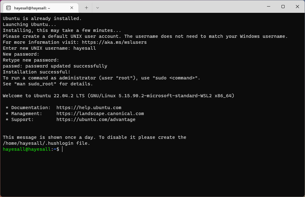
(2) Setup
You will need to set a “UNIX username” and “password.”
- We recommend using your IU username as the username. For example: Alexander uses “hayesall”
- Typing in the password field will not show anything because the text is hidden (you do not want someone to look over your shoulder and easily see your password).
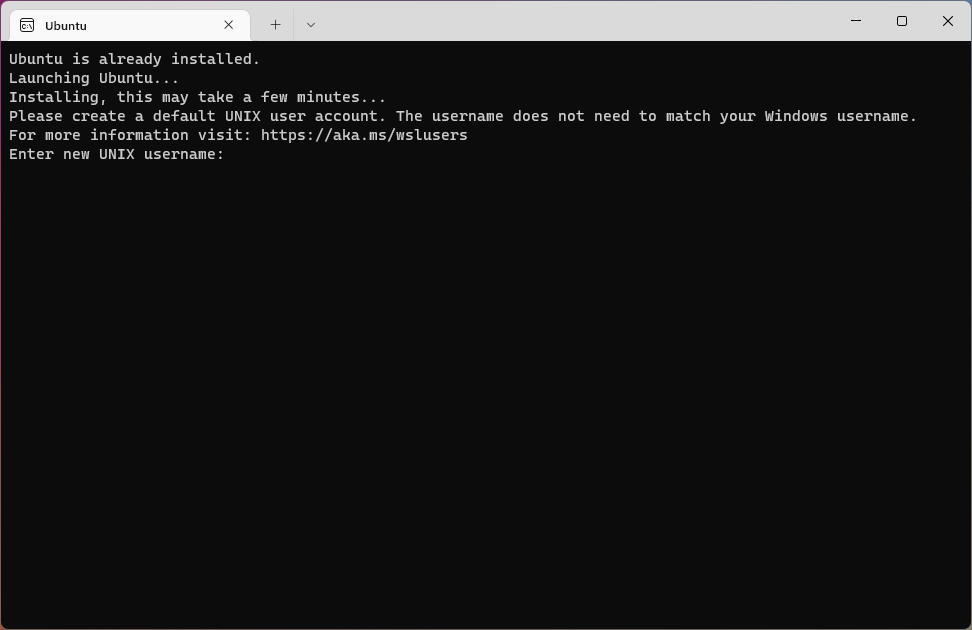
Notice that the area to the right of “New password” and “Retype new password” is empty in the following image. UNIX-like systems handle password fields by not displaying anything: you can type characters but they are are not shown. If you get lost: hold down the Backspace key for a few seconds to clear out anything typed previously.
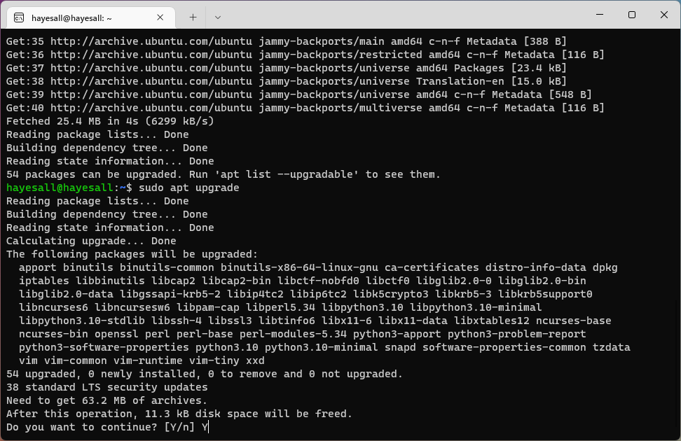
(3) Update, Upgrade, and Install Linux Tools
Similar to the way that Windows has its own set of updates, we need to make sure that our Linux subsystem is up-to-date. Ubuntu has a package manager called apt that helps us here.
Any time we install or upgrade packages, apt will print a message summarizing the changes that are about to take place, and the prompt us for whether we are okay with these:
Do you want to continue? [Y/n]
Briefly skimming the message, typing Y, and pressing Enter is usually going to fine for the workflows we describe in the remainder of the book.
sudo apt update
sudo apt upgrade
We can use this to install any set of packages. git and python3 should be available by default, but we also need venv to manage Python virtual environments:
sudo apt install python3.10-venv
Install Visual Studio Code
📝 Primary Documentation: https://code.visualstudio.com/docs/setup/windows
Follow the VS Code Windows recommendations, and install the WSL extension.
- Download a
.exefrom https://code.visualstudio.com/ - Run the installer
- Open VS Code. A start menu link should be added, allowing you to open the start menu with the Windows key ⊞ Win and type Visual Studio Code.
Install VS Code Extensions
The Extensions Panel is one of the options at the left of VS Code, or can be opened with the Ctrl + Shift + X keyboard shortcut.
The Python Extension and WSL Extension will help us get started. Search and install each by typing the name of the extension in the search bar.
| Python Extension | WSL Extension |
|---|---|
 |  |
Final Check
Open Windows Terminal, then Ubuntu, and check that git, python3, and code are available:
$ git --version
git version 2.34.1

$ python3 --version
Python 3.10.6

$ code --version
1.79.2
Troubleshooting
Example of git missing defaultBranch configuration
$ git init
hint: Using 'master' as the name for the initial branch. This default branch name
hint: is subject to change. To configure the initial branch name to use in all
hint: of your new repositories, which will suppress this warning, call:
hint:
hint:   git config --global init.defaultBranch <name>
hint:
hint: Names commonly chosen instead of 'master' are 'main', 'trunk' and
hint: 'development'. The just-created branch can be renamed via this command:
hint:
hint:   git branch -m <name>
Initialized empty Git repository in /home/hayesall/demo-dir/.git/
Example of the failing venv command
$ python3 -m venv venv
The virtual environment was not created successfully because ensurepip is not
available.  On Debian/Ubuntu systems, you need to install the python3-venv
package using the following command.

    apt install python3.10-venv

You may need to use sudo with that command.  After installing the python3-venv
package, recreate your virtual environment.

Failing command: ['/home/hayesall/demo-dir/venv/bin/python3', '-Im', 'ensurepip', '--upgrade', '--default-pip']
WSL fails to install with WslRegisterDistribution
If a message indicates that the WSL failed to install, for example with a WslRegisterDistribution error similar to the following:
Installing, this may take a few minutes...
WslRegisterDistribution failed with error: 0x80004002
Error: 0x80004002 No such interface supported

Press any key to continue...
A likely fix is to (1) restart the machine, (2) open Windows Terminal in administrator mode (⊞ Win + type “Terminal” + right-click and select “Run as Administrator”), (3) run the wsl --install command again, (4) restart the machine one final time.
WSL starts as the root user
If you open the WSL and see root, similar to this:
root@username:~#
Then an issue occurred when Ubuntu was installing.
Option 1: ubuntu config
- In Ubuntu, check whether your username is in the
passwdfile:
cat /etc/passwd
- Alexander would look for something like:
your_username:x:1000:1000:,,,:/home/your_username:/usr/bin/bash
- In a PowerShell tab, set the default user like this (replacing
your_username):
ubuntu config --default-user your_username
-
Close the Terminal, re-open Ubuntu, and check if it’s fixed.
-
If it is not fixed, try “Option 2”
Option 2: modify the wsl.conf
In Ubuntu, open /etc/wsl.conf with a text editor like nano:
nano /etc/wsl.conf
This configuration should have a [boot] option by default. We will add the Unix username set earlier (replacing the your_username in the following), so the file should look like the following:
[boot]
systemd=true

[user]
default=your_username
Save the changes and exit (e.g.: in nano with Ctrl + O + Enter, then Ctrl + X to exit).
Finally, restart the WSL.
Option 3: re-install Ubuntu
Restart the WSL
Try shutting down the WSL and restarting it.
- Close any Linux (e.g. Ubuntu) tabs in the Terminal
- Open a PowerShell tab
- Run the shutdown command:
wsl --shutdown
exitany Terminal tabs, and close the Terminal- Launch the Terminal again
Upgrade Software
The WSL has its own set of software dependencies that are installed and kept up-to-date separately from the actual Windows operating system.
These commands will ask for your WSL password.
sudo apt update
sudo apt upgrade
Removing and Reinstalling the WSL
Uninstalling then reinstalling an operating system is destructive: it will remove all files, programs, and settings. We will usually recommend this as a last resort if the previous options did not work.
- Close the Windows Terminal, VS Code, and any processes that may have Ubuntu open
- Re-open the Windows Terminal, choosing “PowerShell”
- Uninstall Ubuntu using the
--unregisterflag:
wsl --unregister ubuntu
- Re-install Ubuntu:
wsl --install
Running on macOS
Modern macOS operating systems are descendents of BSD Unix systems. This means that the operating system shares some architectural similarities with the Linux systems that a great deal of the world’s information infrastructure already runs on.
Terminology Specific to macOS
| ⌘ | The ⌘, or “command key” is a symbol on macOS keyboards used for keyboard combinations. Many keyboard combinations include ⌘ for shortcuts, such as ⌘ + c for copying selected text. |
| Dock | The Dock is the location along the bottom of the screen that includes running applications, files, downloads, and applications that have previously been “pinned” to the Dock. |
| Spotlight or Spotlight Search | Spotlight is a convenient way to launch applications. By default it should be possible to access with the keyboard shortcut: ⌘ + SPACE, followed by typing the first few characters of an applications name. For example: open spotlight and type the first few letters of “terminal.” |
| Terminal | macOS has a built-in terminal emulator called “Terminal.” It should be installed by default, may be launched by typing the name into Spotlight and pressing enter, and we recommend pinning it to the Dock for easy access in the future. |
| xcode or XCode | xcode is a macOS application for software and application development on macOS. We will use xcode indirectly by installing it and using some of the developer tools that it includes by default, particularly git. |
Follow Along with the Instructor
Install xcode developer tools
- Open a Terminal
- Pin the Terminal to your Dock (if it is not already)
- Run the xcode installer by typing (or copying & pasting) this into the Terminal:
xcode-select --install
- Restart your machine
Install Visual Studio Code
Follow the Visual Studio Code (VS Code) macOS recommendations.
- Download VS Code
- Click the downloaded file in the web browser downloads
- Drag
Visual Studio Code.appto your Applications folder - Open VS Code by double clicking the icon
- Right click the VS Code icon and pin it to your Dock.
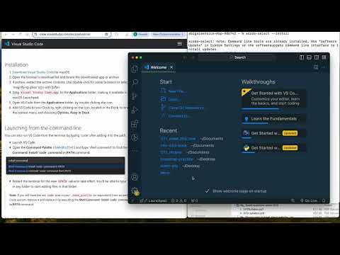
Install VS Code command line tools
- In VS Code, open the command palette with ⌘ + SHIFT + P and type “shell command.”
- Select the option for “Shell Command: Install ‘code’ command in PATH”
- Close VS Code and close the Terminal
Final Check
Check that everything is available in the terminal by running each of the following commands.
If an error message similar to “command not found” appears, double check the installation steps, then ask someone for help if the solution is not obvious.
git --version                   # See "Install xcode developer tools" section
python3 --version
code --version                  # See "VS Code command line tools" section
Troubleshooting
VS Code Permission Errors / Read-only directory
VS Code permission errors are likely caused when VS Code is running out of a read-only directory (e.g. Downloads, Desktop).
- Open VS Code
- Right click and “Show in finder”
- Open another Finder window with your Applications directory
- Drag the icon from the old location to the Applications directory
Running on ChromeOS
ChromeOS is an operating system initially released on 2011. By default, ChromeOS supports a Chrome web browser as the primary frontend for users to interact with—thereby giving access to websites and web applications. In 2016, support for running Android applications was added. In 2018, a virtual machine based on Debian Linux was added, making it easier to run any application which could run in a Linux environment.1
Enable Developer Mode and Linux Environment
This guide follows the ChromeOS Linux Setup Documentation
- Open “Settings” > “Advanced” > “Developers” > “Turn on” Linux Development Environment
- Restart your Chromebook
- Open “Terminal” and “Pin” it to your shelf
Install Development Environment
Open the Terminal and run the apt install command as follows:
sudo apt install git python3 python3-dev python3-venv
Install VS Code
Follow the VS Code Linux recommendations.
- Download the
.debpackage from the website - Move the package into the Linux environment using the “Files” program
- Open the Terminal and install with:
sudo apt install ./<file>.deb
Footnotes
ChromeOS itself is a Linux environment, and you can access its “crosh” shell using ctrl + alt + t. Since it’s a Linux-based environment underneath, there is an alternative way to access the internals with a program called crouton. crouton makes it possible to install Ubuntu or Debian, or install a complete Linux desktop. However, we consider this approach to be more advanced than is necessary for the other material here.
Running on Ubuntu Desktop
This guide is for Ubuntu Desktop, if you’re using the Ubuntu that ships with the Windows Subsystem for Linux (WSL), then check the Windows guide instead.
Ubuntu is a ubiquitous Linux distribution known for being a welcoming distribution to newcomers, but also having all the tools available for when you want to strap a jet engine onto it. One might even say that Ubuntu is the Python of Linux distributions.
Install Dependencies
Similar to the ChromeOS guide, the following should cover everything we need for this course.
sudo apt install git python3 python3-dev python3-venv
Install VS Code
Follow the VS Code Linux recommendations.
- Download the
.debpackage from the website - Open the Terminal and install with:
sudo apt install ./<file>.deb
I211 Unit 1: Foundations
In I210, we learned the foundations of programming using Python. The goal was to write a computer program.
In I211, the goal is to write multiple computer programs, using multiple languages and an upgraded workflow, that work together as a web application.
The structure of our programs will change. In I210, you likely learned programs contain these three steps:
INPUT
PROCESSING
OUTPUT
In I211, programs will be upgraded to at least this:
INPUT
  (+ format input to be usable within our program + data cleaning)
PROCESSING
  (+ data validation)
OUTPUT
  (+ more complex data + databases)
What are our goals in I211?
The goal is to be able to create a full stack web application, which will require us to address the following:
-
Design: How do we turn an idea or a feature into a program?
-
Code: Write better code, manage code changes, and share code with others.
-
Test: What are edge cases and how do we test for them? How do we prevent bad or malicious data entry? How do we ensure that your code will work in another environment?
-
Release: How do we move code from one environment to another?
We will also upgrade our workflow
Your workflow will not just be running Python in VS Code, it will involve multiple technologies working together. We will begin by introducing the command line, and technologies that support web development, such as Git and Github.
We will then review Python with the goal of introducing testing of our code, working with GitHub repositories, and eventually installing Flask (a popular Python-based web application framework).
Linux/Unix-like Environments
Unix-like Environments (sometimes written “*nix environments”) refer to any of a family of operating systems that were either derived or based on the early PDP and Unix operating systems of the 1960s and 1970s. Today when people refer to Unix-like Environments, they typically mean a macOS or Linux machine.
Nonetheless, there are many systems that share similarities with the two:
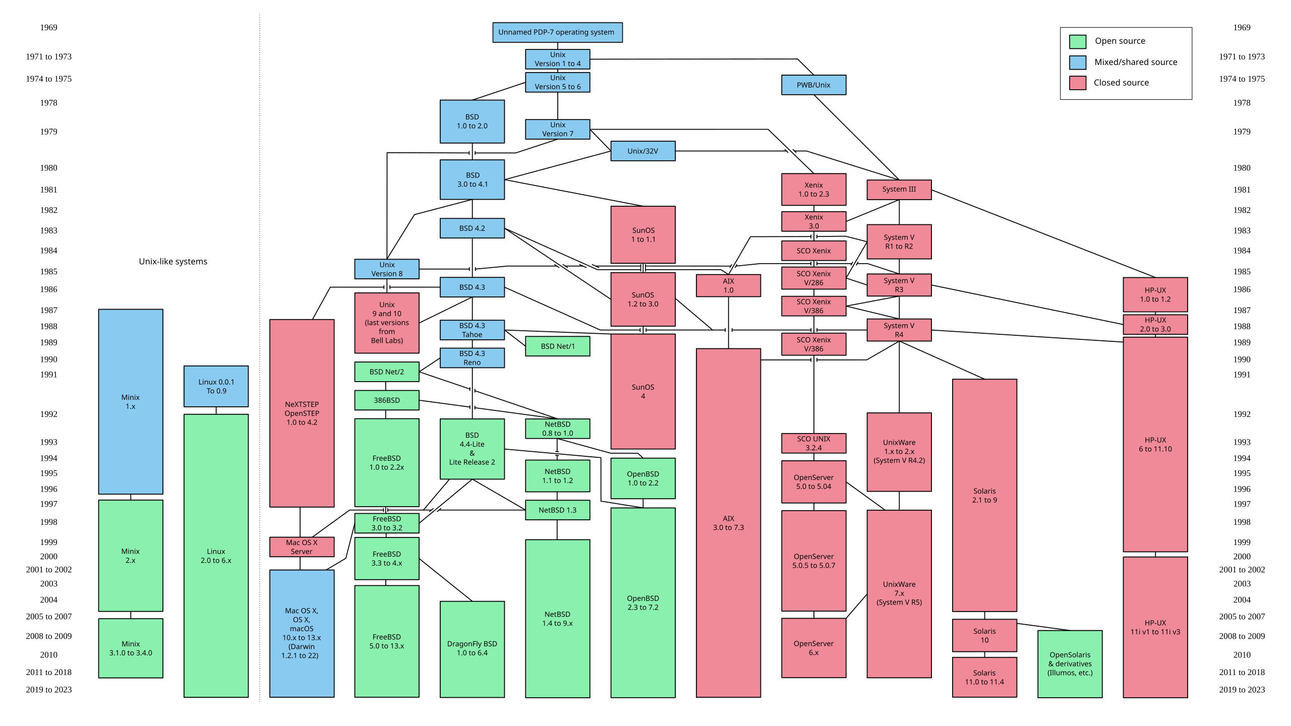
Other operating systems developed in parallel: such as the Windows operating systems that was based on DOS (another early operating system, and an acronym for “Disk Operating System”). Understanding the details of an operating system may be important for specific tasks—if we were developing video games and planning for them to be played on Windows, we would want to better understand details of the Windows platform.
However, Unix-like environments—and Linux environments specifically—are prolific across a range of computing problems. When a user navigates to a web page, their browser (e.g. Firefox, Chrome, Edge) is almost certainly communicating with several other computers running some flavor of Linux.
“The Cloud” sounds like a deific object, but in reality the cloud is a room full of machines running virtual machines inside of them: launching into existence just long enough to accomplish some task before exporting some data and disappearing entirely. In other words: “The Cloud” is referring to to a series of Unix-like environments.
We’ll focus on three key skills in this section:
-
Familiarity with File Systems. A File System organizes content into files and folders (which we’ll start referring to as “directories” soon).
-
Knowing enough about Terminals and Shells to move around, launch programs, and be productive. Most modern operating systems have a graphical shell called a “Desktop” with buttons—but an interface supporting text input and text output is frequently the quickest (or only) means of accomplishing computing tasks.
-
Having enough knowledge of Process Management to launch processes, wait on them to complete, debug them, or end them if necessary.
We will practice working in Unix-like environments here. macOS users already have this environment. Windows users should use the WSL (Windows Subsystem for Linux) to maintain a seemless experience with the material.1
Perfectly Spherical Operating Systems
An operating system is a program that manages hardware or computer resources.
Mainstream operating systems are built around a hierarchical tree structure created out of directories (folders) and the files inside of the directories. A file stories data, and directories might be used to group related data together in some logical way.
Directories
There exists a root directory. That root directory contains other directories. These two facts create a parent-child relationship between directories.
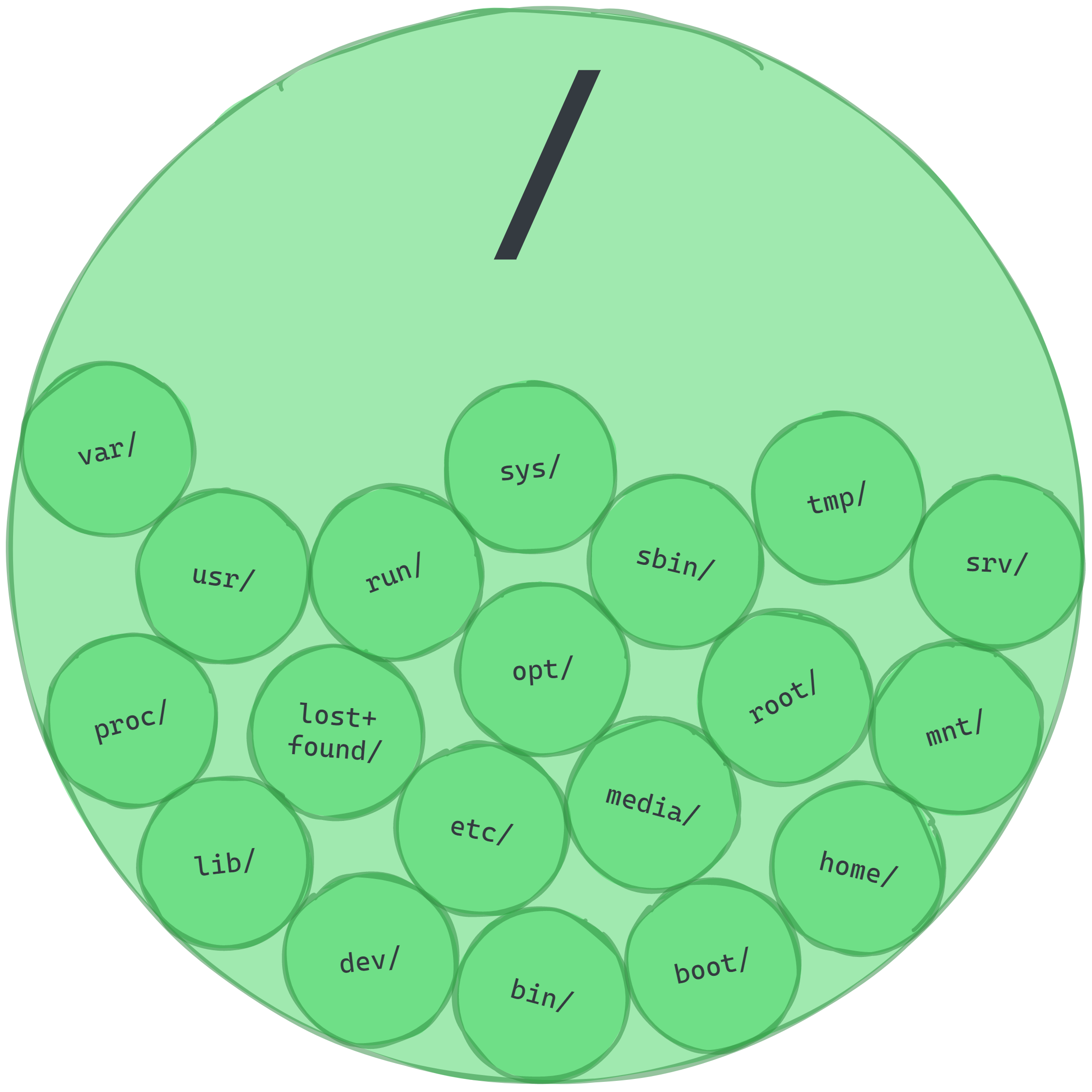
Every child can have children of its own: but every child has one and only one parent.2 This means that the parent-child relationships could (in principle) extend like nesting dolls infinitely far down into folders-inside-of-folders-inside-of-folders:
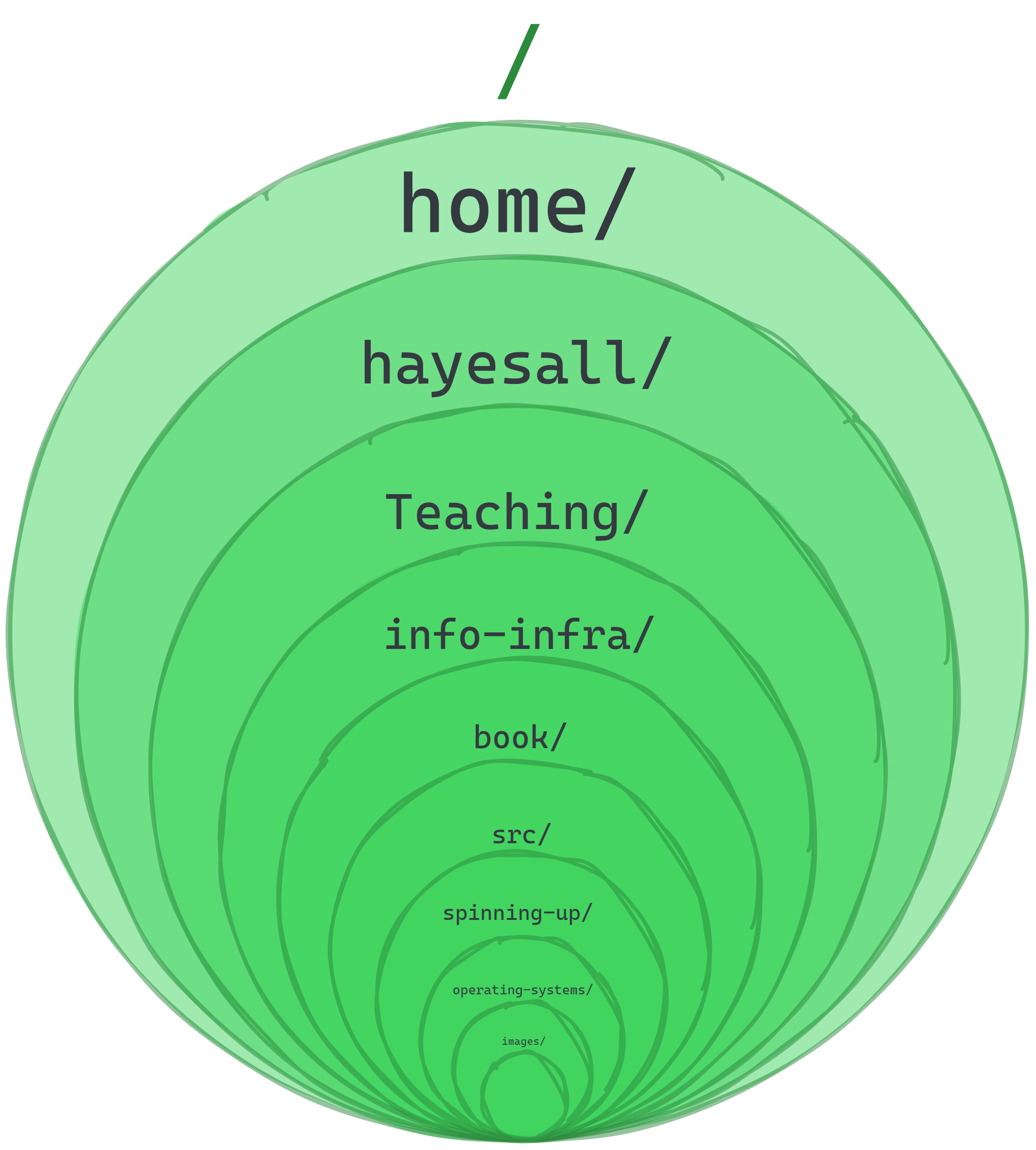
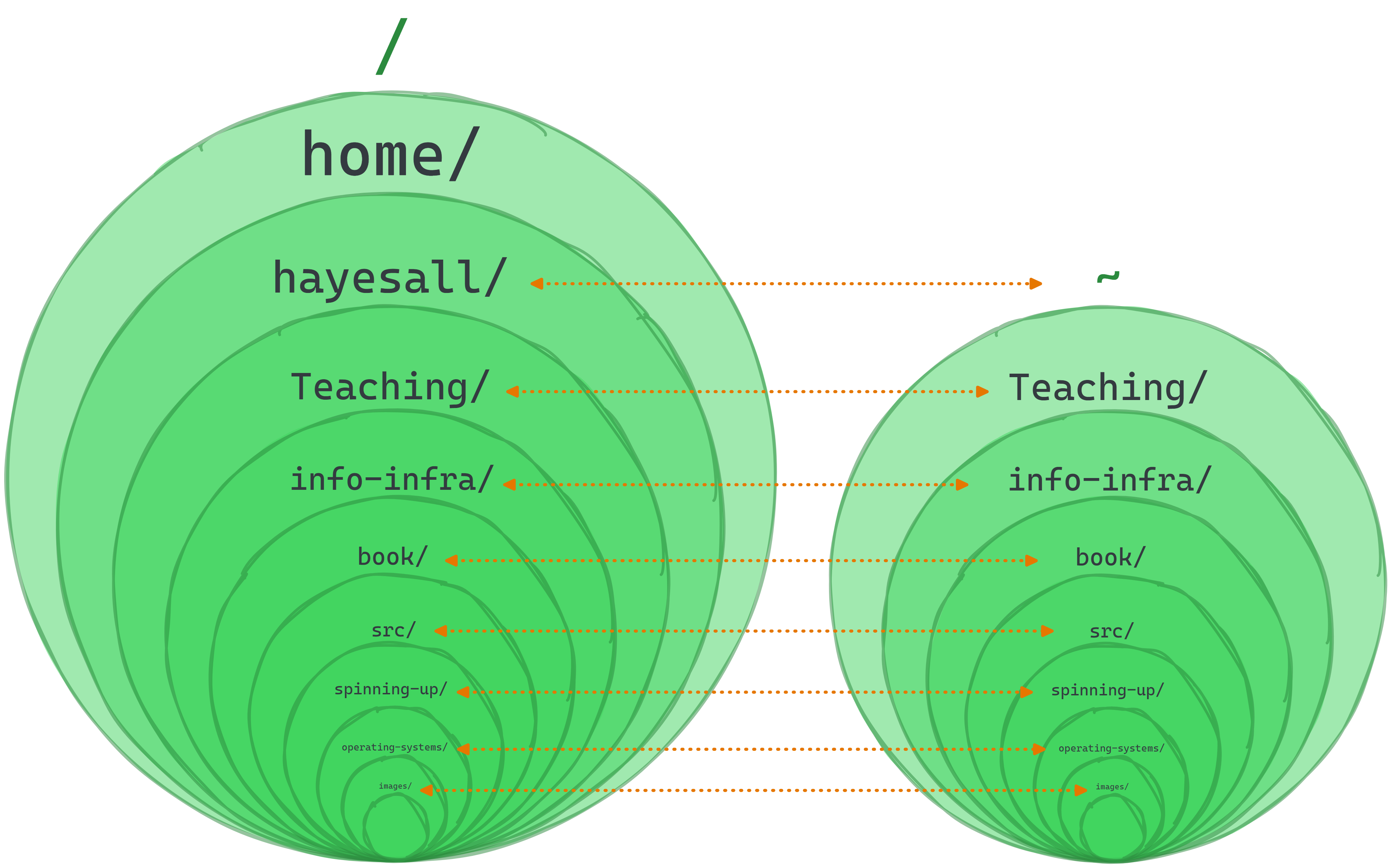
Assume everything above is in its place, and give a special name using the tilde ~ to represent the home directory. Everything from earlier is still true, but we’ve constrained the universe where only a specific part of it is relevant. As Unix users, our actions are almost always relative to our home directory: the lower levels do exist, meaning the levels closest to “root” or /, but they’re safe to ignore during most day-to-day activities:
The Same Person with Many Faces
On each operating system that you’re likely to encounter: there exists some concept of “root” and “home.” They look slightly different though:
macOS /Users/hayesall/Linux /home/hayesall/Windows C:\Users\hayesall\Each has slightly different behavior, but most programs will assume a home directory
~exists for the user, and that the home directory and (by transitivity) everything inside of it belongs to the user.
Follow Along with the Instructor
Practice with the instructor. Not an exact replacement for the written directions below.
- Become comfortable with the command line interface and the structure of Linux/Unix file systems
Files and Directories
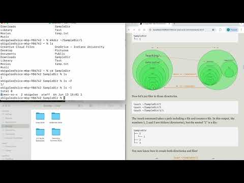
Open your Terminal (Mac) or WSL (Windows) to follow along.
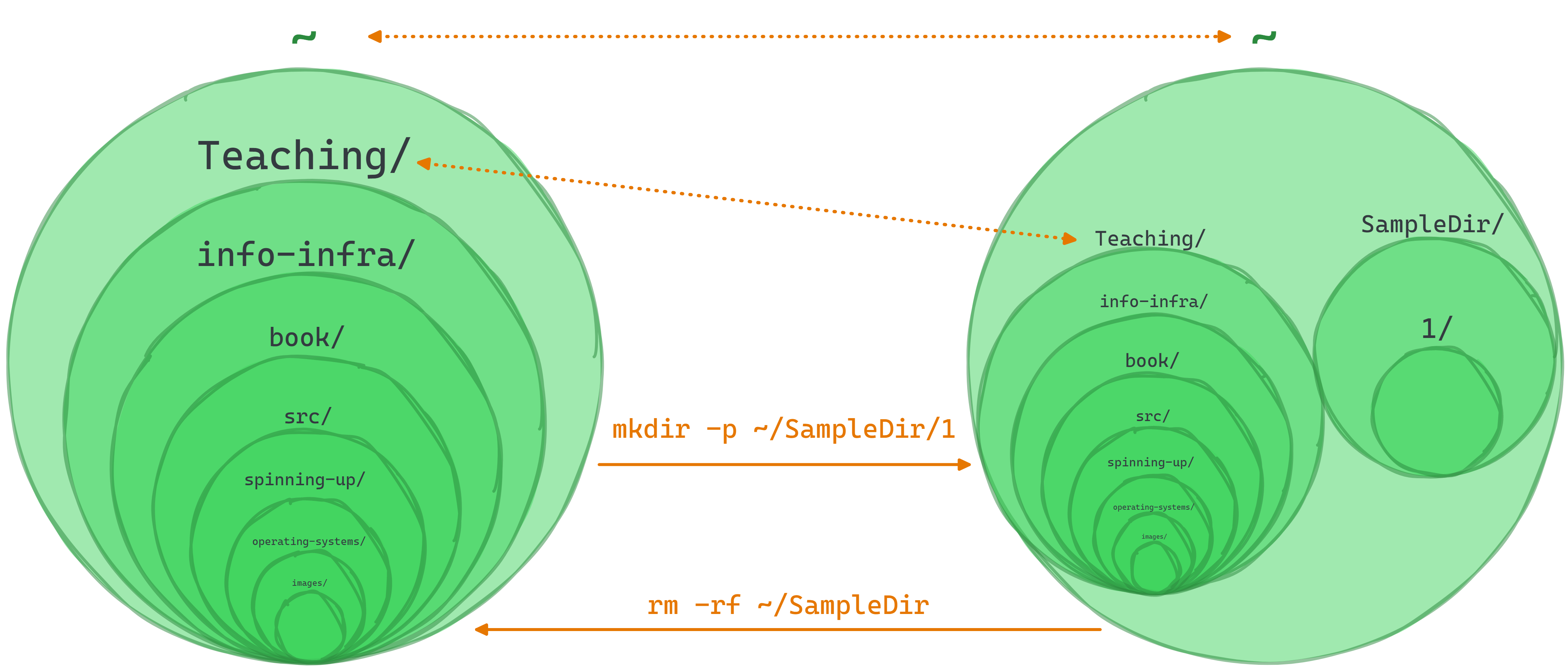
Let’s create a new directory called SampleDir in the user’s home directory, and put another directory called 1 inside of SampleDir.
- Everytime you see
~a tilde, it means the user’s home directory. - A forward slash
/indicates a directory.
mkdir ~/SampleDir
mkdir ~/SampleDir/1
This creates the following structue; a directory called “SampleDir” containing another directory called “1”:
SampleDir
└── 1
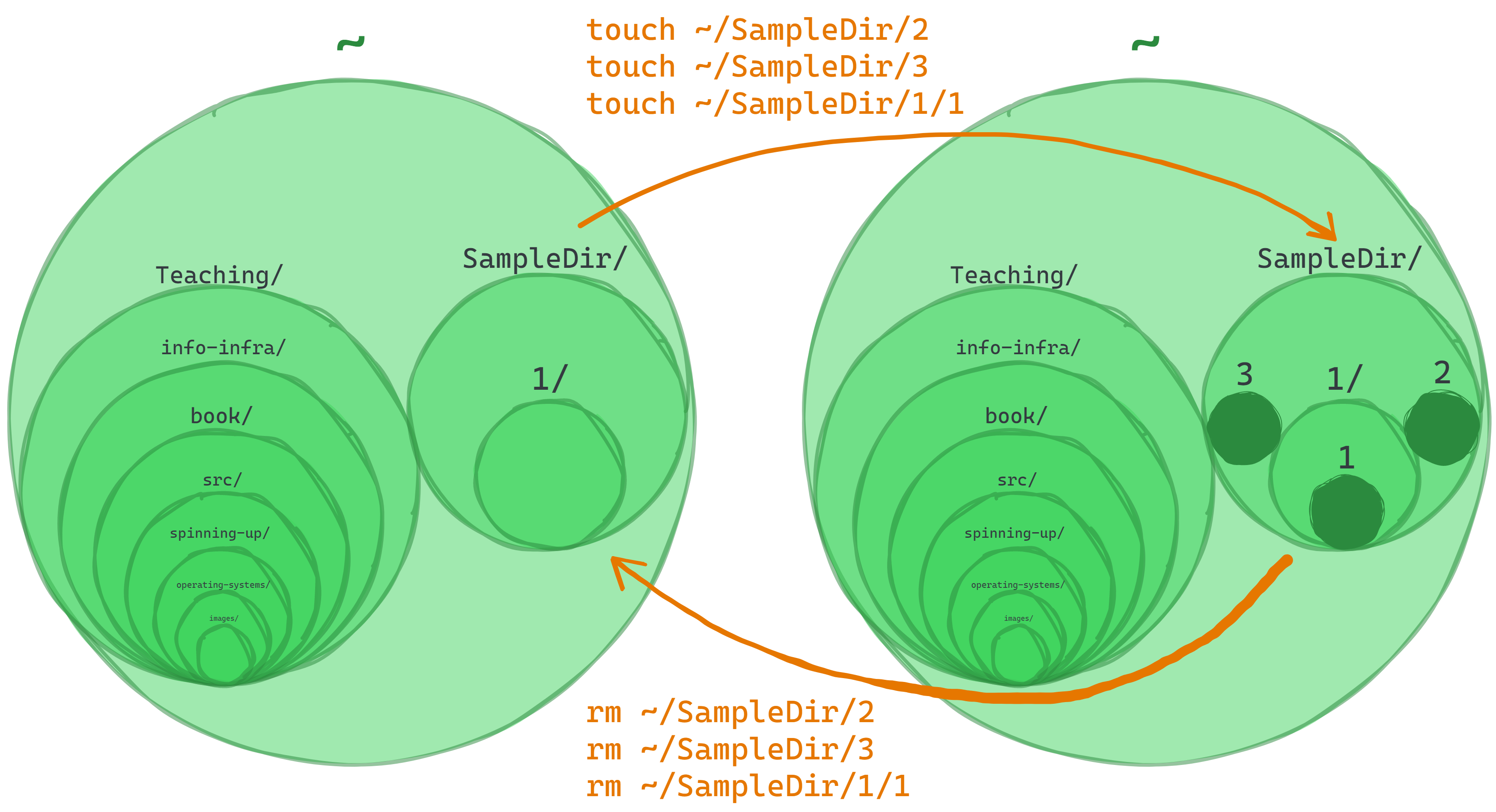
Now let’s put files in those directories.
touch ~/SampleDir/2
touch ~/SampleDir/3
touch ~/SampleDir/1/1
The touch command takes a path including a file and creates a file. In this output, the numbers 1, 2 and 3 are folders (directories), but the nested “1” is a file:
SampleDir
├── 1
│  └── 1
├── 2
└── 3
You now know how to create both directories and files!
Some basic Unix commands
It might help to think of the next few commands as controlling a cursor.
In a graphical shell (how you’ve probably used computers previously), one can use the mouse to move a cursor on a screen, and click/double-click to move into folders. Typically: there is also some text providing feedback for where one is.
Where are you?
pwd » Print Working Directory
For example: pwd for Alexander shows /home/hayesall
What is in here, or there?
ls » List files in the current directory
ls is also a program which takes a file path as an argument. For example: ls /home/hayesall/ will show the files in that directory.
Linux distributions often avoid polluting the user’s home directory with unnecessary files and folders. Therefore, if you’re on the Windows Subsystem for Linux, you will not see anything by default:
$ ls /home/hayesall
On a Mac, you’re likely to see familiar folders such as “Desktop”, “Documents”, or “Downloads”.
Dollar signs?
$/ Percent signs?%In technical writing, authors often use a dollar sign
$or percent sign%to communicate when operations are done in a terminal or text shell. The$is a common prompt token indicating that the shell is ready for the next command. The default on Linux typically looks like:hayesall@hayesall:~$, or likeebigalee@sice ~ %on macOS.The takeaway: do not copy the dollar sign when you’re following along, you’ll probably get something like:
$: command not found.
There are files in the home directory, but they are hidden files that start with a period .. These dotfiles are often used for configuration in Unix-like environments.
To view hidden files, you can add an option called a flag, to your command. A flag modifies the behavior of a command, giving you access to additional functionality when needed. For example:
ls -a » List files in current directory, also showing hidden files
$ ls -a ~
.  ..  .bash_history  .bash_logout  .bashrc  .local  .profile  .viminfo
ls -l » List files in current directory, in long listing mode
$ ls -l
total 0
The long listing for files gives information on resource information (d for directory, or - for file) file permissions (is it readable r, writable w, or executable e?), ownership, file size (in bytes), and the last modified timestamp.
But since our files are hidden, we need to use both the -a and the -l flags:
$ ls -a -l
total 36
drwxr-x--- 3 hayesall hayesall 4096 Jun 13 10:01 .
drwxr-xr-x 5 root     root     4096 May 15 12:38 ..
-rw------- 1 hayesall hayesall 1223 Jun 12 15:16 .bash_history
-rw-r--r-- 1 hayesall hayesall  220 May 15 12:38 .bash_logout
-rw-r--r-- 1 hayesall hayesall 3771 May 15 12:38 .bashrc
-rw------- 1 hayesall hayesall   20 Jun 12 14:03 .lesshst
drwxrwxr-x 3 hayesall hayesall 4096 May 15 12:39 .local
-rw-r--r-- 1 hayesall hayesall  807 May 15 12:38 .profile
-rw------- 1 hayesall hayesall  756 May 15 12:41 .viminfo
How do we learn more?
We could go on-and-on about ls, as there are literally thousands of variations just on the ls command: all configured through flags.
No one expects you to have every single variation on every single command memorized. If we were to allocate space for every variation: this chapter would meander on for thousands of pages.
But we do expect you to be able to look up the details when you need them. man pages, or manual pages are one of the best ways to look up this information without leaving the terminal.3
$ man ls
(Hint: Type Q to quit out of a man page.)
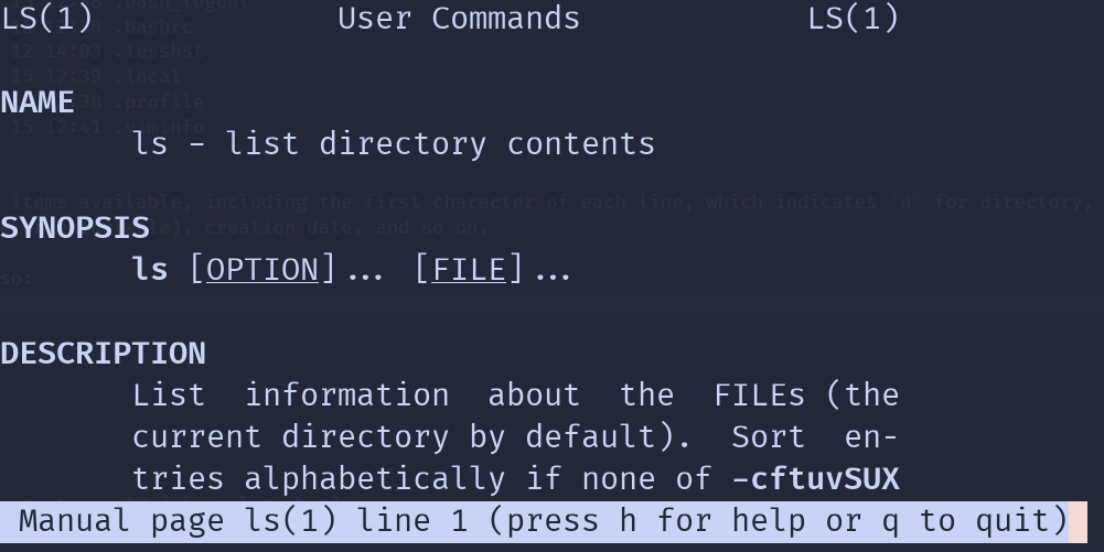
This chapter will cover what we feel are the absolute essentials: a self-contained, minimal set of commands that you need to be productive and accomplish your daily work. But there is no substitute for continuous learning and self-improvement.
Make Directories
mkdir directory » Make directory
On Unix systems, we will usually recommend you avoid using spaces. When typing commands, spaces are used to separate each part of command. So to create a directory:
$ mkdir daily-work
… will create a daily-work directory, but:
$ mkdir Daily Work
… creates two directories: Daily and Work.
$ ls
Daily  Work  daily-work
Remove Directories
rmdir directory » Remove directory
If we make a directory that we didn’t intend, or want to clean up, rmdir removes it:
$ rmdir Daily
$ rmdir Work
Make Files
touch file » Create a new file
Technically the touch command modifies timestamps, but its effect is to create new files if they do not exist:
$ touch notes.txt
$ ls
daily-work  notes.txt
One can also chain paths together using the / to create files inside of directories:
$ touch daily-work/step01.txt
$ touch daily-work/step02.txt
$ ls daily-work/
step01.txt  step02.txt
Remove Files
rm file » Remove, delete
⚠️ Caution! ⚠️
Most graphical user interfaces with friendly clickable buttons have Trash or a Recycling Bin. When the user deletes something, it goes in the bin, then the user must explicitly opt into emptying the trash.
Unix/Linux does not do this. When you tell your shell to remove something: it is gone, and there is no undo button.
When one can create files, one also needs to be able to remove them.
$ rm daily-work/step01.txt
$ ls daily-work/
step02.txt
But if one tries to remove something with something else inside of it: it’s an error:
$ rmdir daily-work/
rmdir: failed to remove 'daily-work/': Directory not empty
$ rm daily-work/
rm: cannot remove 'daily-work/': Is a directory
To remove a directory, everything inside of it, (and potentially everything inside everything that is inside of it—and so on): one must recursive remove with the -r flag:
$ rm -r daily-work
$ ls
notes.txt
Moving around inside the terminal:
cd path » Change Directory
cd is a program that takes a directory name as an argument, and changes into that directory. In a graphical file explorer, this is like double clicking a folder to navigate inside that folder.
If one creates a Classes directory with an i211 directory inside of it:
$ mkdir -p Classes/i211
Then the result is a file hierarchy. Some systems have a tree command (on Ubuntu/WSL: sudo apt install tree) that visualize these:
$ tree Classes/
Classes/
└── i211
Calling cd Classes/ will change your working directory. On Alexander’s: the absolute path becomes /home/hayesall/Classes, or relative path against the home directory is ~/Classes:
$ cd Classes
$ ls
i211
What happens if we type cd with no arguments?
$ pwd
/home/hayesall/Classes
$ cd
$ pwd
/home/hayesall
Therefore, you can always get home by typing cd with no arguments, or typing cd ~ (where the tilde ~ expands to your home directory).
Dot and Double Dot: The Relative Here and There
ls . » list files in here
cd .. » go there, to the parent directory
Every directory in a Unix-like system has two special resources inside of it: . and ...
The terminology for what these two things are called is inconsistent, so Alexander refers to them as here . and there .., because no matter where you are in some virtual space: there is always a here and a there. One may traverse from point A to point B by traversing the relative spaces between the two points.
~- the home directory.- the current directory..- the parent directory../..- the grandparent directory../../..- the great-grandparent directory
For example, if one creates five directories nested inside one another:
$ mkdir -p A/B/C/D/E
$ tree A
A
└── B
    └── C
        └── D
            └── E
… then one may reach C by with:
$ cd A/B/C
$ ls
D
… and then return home by following the chain of parent directories:
$ cd ../../..
$ ls
A
Since every directory has a . representing the current location on the file system, we can now think of ls as having the current directory . as a default argument. ls and ls . function the same:
$ ls .
A
From the rules of here and there, arbitrary complexity may be reached:
$ cd ./A/B/C/../C/../../B/././.
$ ls .
C
But even though these can be combined toward arbitrary complexity: one should strive to organize one’s file system in a logical way to avoid this. For example, in a web development project with hypertext markup language (HTML) and cascading style sheets (CSS), it’s common to organize files and directories like this:
$ mkdir -p some-html-project/css
$ touch some-html-project/{index,other}.html
$ touch some-html-project/css/main.css
$ tree some-html-project
some-html-project/
├── css
│   └── main.css
├── index.html
└── other.html
In this file hierarchy:
- when
index.htmlreferences a CSS file, the relative path is./css/main.css - if
index.htmlneeds a link toother.html, the relative path is./other.htmlsince both are in the same directory
Which way to the root? Up ⬆️ or Down ⬇️ ?
Are you descending to the root, or ascending to the root?
Many will say ascending up to the root, and that
cd ..is going up a directory. This is an artifact of how computer science textbooks historically drew trees: with the root node at the top and the leaf nodes at the bottom.

But this choice is arbitrary: it depends on how one views or visualizes hierarchy. Is it a foundation which everything rests upon? Or is it the peak for one to climb to, from which all authority flows?4

Edit a file in the command line
nano filename » Edit a file
nano is a simple text editor letting you write text inside of files without leaving the command line.
touch ~/Classes/i211/practice.txt
nano ~/Classes/i211/practice.txt
A basic interface will fill the space, typed text becomes part of the file:
- the cursor can only be moved using the keyboard, not the mouse
- when you are done you will run a set of commands to save, exit and return to the command line prompt
Control + X    (Exit)
Y              (Save modified buffer Yes No)
[Return]       (Return/Enter key will go back to the cursor)
Quickly view a file
cat filename » Concatenate the file to the terminal, showing the content
less filename » Preview the file
If you want to see if the file saved, or just check what is in a file, there are several ways to print out the contents in the command line.
If the file isn’t too long:
$ cat ~/Classes/i211/practice.txt
In i211, we are practicing with Unix and with
the nano text editor.
If you want a better interface, less is a terminal pager program where you can page up and down in the file, and use Q to quit back to what you were previously doing.
less ~/Classes/i211/practice.txt
q
Renaming, Moving, and Copying
mv old-name new-name » move or rename a resource from one name to another
cp some-name other-name » copy a resource from one place to another
Moving and renaming from the perspective of a file system are really the same fundamental operation: every file or directory has a name, and we’re changing that name from something to something else.
For example, if we accidentally type otes.txt when we intended to write notes.txt:
$ cd ~/Classes/i211
$ touch otes.txt
$ ls
otes.txt  practice.txt
Then we can rename the file by moving otes.txt to a new name: notes.txt:
$ mv otes.txt notes.txt
$ ls
notes.txt  practice.txt
Copying works the same way, but if the file contained content, then that content would be copied to a new location. Since practice.txt contained some text, copying the file somewhere should have the same text:
$ cp practice.txt assignment.txt
$ cat assignment.txt
In i211, we are practicing with Unix and with
the nano text editor.
If we want to copy a directory and everything inside of it—e.g. when copying files in a directory for a new class—we can modify how cp behaves with the recursive -r flag.
$ cd ~/Classes
$ ls
i211
$ cp -r i211 i210
$ tree ~/Classes
/home/hayesall/Classes
├── i210
│   ├── assignment.txt
│   ├── notes.txt
│   └── practice.txt
└── i211
    ├── assignment.txt
    ├── notes.txt
    └── practice.txt

2 directories, 6 files
Cleanup, Review, and Practice
We will not re-use any of the files or directories from this chapter, so everything from today is safe to remove:
$ rm -r ~/Classes
We’ll review and share some final notes before going into practice.
Terminal Shortcuts
Many text shells (and command line interface programs) come with these helpful features:
- Tab Completion - once the command or filename is typed in far enough that it is unique among possible names it could be, you can hit Tab ↹ on your keyboard and the filename will be completed for you
- History - commands are saved in your history. To cycle back to previous command: use the up arrow key ↑ on your keyboard as many times as needed
These two features are then made part of a host of keyboard shortcuts for text editing, autocompleting, and history searching.
🍎 Terminal Shortcuts on macOS
macOS shortcuts vary slightly depending on the shell that came with your computer. We list variants in the table, or you can use the dropdown menus at the top to check for your computer.
| Shortcut | macOS variant | Description |
|---|---|---|
| Tab ↹ | complete command | |
| ^ Ctrl + L | like running the clear command | |
| Alt + ↵ Enter | Function + F | toggle full screen terminal |
| ↑ / ^ Ctrl + P | cycle through previous commands | |
| ↓ / ^ Ctrl + N | cycle through next commands | |
| ^ Ctrl + C | interrupt signal | |
| ^ Ctrl + ⇧ Shift + T | ⌘ Cmd + T | new tab |
| ← | one character left | |
| → | one character right | |
| ^ Ctrl + ← | ⌥ Option + ← | one word left |
| ^ Ctrl + → | ⌥ Option + → | one word right |
| Alt + ← Backspace / ^ Ctrl + W | delete last word | |
| ^ Ctrl + A | text stArt | |
| ^ Ctrl + E | text End | |
| ^ Ctrl + K | “kill” text to end of line into a buffer | |
| ^ Ctrl + Y | “yank” from buffer to paste | |
| ^ Ctrl + D | “end of transmission”, like running exit | |
| ^ Ctrl + R | reverse history search |
Pathnames
The file structure we learned here today is repeated throughout the coding world, and understanding how pathnames work is important to creating projects later in the course.
A pathname is, you guessed it, what pwd prints out in our terminal. It’s a text representation of the data structure used for organizing files and directories. And once you see it, you’ll see it everywhere there is code.
Even as a URL in your browser!
Review
Commands from this chapter have two main uses: those that give us information about the state of our system,
| command | description |
|---|---|
pwd | print working directory |
ls | list files |
cat file | show file’s content |
less file | preview the file with a pager |
ls -a | list files and hidden files |
ls -l | list with details |
tree directory | visualize a file tree |
and those that mutate (create, remove, update) the system to fit our needs:
| command | description |
|---|---|
touch file | create a file |
mkdir directory | make a directory |
mkdir -p dir/with/paths | make nested directories |
rm file | remove a file |
rm -r path | recursive remove |
rmdir directory | remove a directory |
cd path | change directory |
nano file | edit text in a file |
mv old-name new-name | move or rename a resource |
cp some-name other-name | copy a file |
cp -r some-name other-name | copy recursively |
Practice Exercises
01 Simple Hierarchy
Recreate this file hierarchy using mkdir, touch, and maybe cd
unix-practice
└── f01
   ├── f1.txt
   └── f2.txt
Possible Solution
mkdir unix-practice
mkdir unix-practice/f01
touch unix-practice/f01/f1.txt
touch unix-practice/f01/f2.txt
Alternate Solution
The mkdir -p variation expands paths that do not exist. Braces {} and commas are expanded by the shell, so the command: touch {01,02}.txt expands into into creating two files that end with a .txt extension.
mkdir -p unix-practice/f01
touch unix-practice/f01/{f1,f2}.txt
02 Website Hierarchy
Static websites may be built from hypertext markup language (HTML), cascading style sheets (CSS), and JavaScript (JS). Sites typically have extra configuration files (e.g., robots.txt, Sitemaps) to help online services like search engines index the site. Reproduce the following website template using mkdir, touch, and possibly cd.
unix-practice
└── some-empty-site
   ├── css
   │  ├── main.css
   │  └── reset.css
   ├── index.html
   ├── js
   │  └── main.js
   ├── robots.txt
   └── sitemap.xml
Possible Solution
mkdir unix-practice/some-empty-site
mkdir unix-practice/some-empty-site/css
mkdir unix-practice/some-empty-site/js
cd unix-practice/some-empty-site/css
touch main.css reset.css
cd ..
touch index.html robots.txt sitemap.xml
touch js/main.js
cd ../..
Alternate Solution
mkdir -p unix-practice/some-empty-site/{css,js}
touch unix-practice/some-empty-site/css/{main,reset}.css
touch unix-practice/some-empty-site/js/main.js
touch unix-practice/some-empty-site/{index.html,robots.txt,sitemap.xml}
03 Python Hierarchy
A Python package is a collection of Python code and configuration files informing a package installer (e.g. pip) where code is and how that code is loaded in order to be used in a downstream dependency. Reproduce the file hierarchy of a typical Python project inside the unix_practice folder, using mkdir, touch, and cd as needed:
unix-practice
└── empty-python-project
   ├── my_project
   │  ├── __init__.py
   │  ├── __main__.py
   │  └── tests
   │     ├── __init__.py
   │     └── test_setup.py
   ├── pyproject.toml
   ├── README.md
   └── requirements.txt
Possible Solution
mkdir unix-practice/empty-python-project
mkdir unix-practice/empty-python-project/my_project
mkdir unix-practice/empty-python-project/my_project/tests
cd unix-practice/empty-python-project
touch pyproject.toml
touch README.md
touch requirements.txt
cd my_project
touch __init__.py
touch __main__.py
cd tests
touch __init__.py
touch test_setup.py
cd ../../../..
Alternate Solution
mkdir -p unix-practice/empty-python-project/my_project/tests
touch unix-practice/empty-python-project/{pyproject.toml,README.md,requirements.txt}
touch unix-practice/empty-python-project/{my_project,my_project/tests}/__init__.py
touch unix-practice/empty-python-project/my_project/__main__.py
touch unix-practice/empty-python-project/my_project/tests/test_setup.py
04 Julia Hierarchy
Julia is a relatively new programming language developed with scientific programming in mind. Reproduce the file hierarchy used in a typical Julia project:
unix-practice
└── empty-julia-project
   ├── docs
   │  ├── make.jl
   │  └── Project.toml
   ├── Project.toml
   ├── README.md
   ├── src
   │  ├── main.jl
   │  └── types.jl
   └── test
      ├── Project.toml
      ├── runtests.jl
      └── test_types.jl
Possible Solution
mkdir unix-practice/empty-julia-project
cd unix-practice/empty-julia-project
mkdir docs src test
touch Project.toml README.md
cd docs
touch make.jl Project.toml
cd ../src
touch main.jl types.jl
cd ../test
touch Project.toml runtests.jl test_types.jl
cd ../../..
Alternate Solution
mkdir -p unix-practice/empty-julia-project/{docs,src,test}
touch unix-practice/empty-julia-project/README.md
touch unix-practice/empty-julia-project/{.,docs,test}/Project.toml
touch unix-practice/empty-julia-project/docs/make.jl
touch unix-practice/empty-julia-project/src/{main,types}.jl
touch unix-practice/empty-julia-project/test/{runtests,test_types}.jl
05 Java Hierarchy
Java is known for using deeply-nested paths. (Hint: mkdir -p creates all intermediate paths, allowing you to string together several/different/directories at once). Reproduce a Java file hierarchy:
unix-practice
└── empty-java-project
   ├── build.gradle
   ├── README.md
   └── src
      ├── main
      │  └── java
      │     └── com
      │        └── hayesall
      │           └── Main.java
      └── test
         └── java
            └── com
               └── hayesall
                  └── Test.java
Possible Solution
mkdir -p unix-practice/empty-java-project/src/main/java/com/hayesall
mkdir -p unix-practice/empty-java-project/src/test/java/com/hayesall
cd unix-practice/empty-java-project
touch build.gradle README.md
touch src/main/java/com/hayesall/Main.java
touch src/test/java/com/hayesall/Test.java
cd ../..
Alternate Solution
mkdir -p unix-practice/empty-java-project/src/{main,test}/java/com/hayesall
touch unix-practice/empty-java-project/{build.gradle,README.md}
touch unix-practice/empty-java-project/src/main/java/com/hayesall/Main.java
touch unix-practice/empty-java-project/src/test/java/com/hayesall/Test.java
06 Text Trip Planning
Now that we’re comfortable (1) creating files and directories, and (2) navigating with cd; let’s add file editing with nano into our workflow.
We’re going on a trip. Let’s create files and directories to house our planning notes. Start with:
mkdir ~/TripPlanning
then:
- navigate into the
TripPlanningdirectory - create a file called
snacks.txt - edit
snacks.txt, adding your favorite snacks - save and exit
nano
Now add two directories: Destinations and Ideas.
TripPlanning
├── Destinations
├── Ideas
└── snacks.txt
Create files in Destinations and Ideas for some places you want to go and some ideas for what you might do while you’re there. Here are some ideas if you’re stuck:
TripPlanning
├── Destinations
│  ├── Gershwin-Theatre.txt
│  ├── Met-Museum-of-Art.txt
│  └── Statue-of-Liberty.txt
├── Ideas
│  ├── drag-brunch.txt
│  └── roller-skating.txt
└── snacks.txt
Self-reflection:
- Can you successfuly add some text to each
.txtfile using nano? - Can you move up a level from
Ideasback toTripPlanning? - Can you change from
IdeastoDestinationsin one line? - How about getting back home?
When you have completed the practice, you can delete the practice directory:
rm -rf ~/TripPlanning
Exit the terminal when you’re finished, either by:
- typing:
exit+ ↵ Enter - or send an end-of-transmission ␄ with: ^ Ctrl + D
Stuck?
Chat with us on Discord, in office hours, or send us an email!
Footnotes
Most recent Windows machines support PowerShell by default. We will always recommend “getting to know your own machine,” and PowerShell is a great skill to pick up as you learn more about Windows. However: PowerShell has a separate suite of programs for common tasks like file creation (since Windows assigns different semantic meaning to “file extensions”), so it is outside the scope of what we intend to cover here.
There is an exception to the rule of “everything has one and only one parent”, but it violates how people often think about physical objects. In a physical file system: a sheet of paper cannot exist in two folders at the same time, because it’s not possible for the same thing to be in two places at once. Computers do not have this restriction: software is not bound by the finicky constraints of reality. If one first allows wormholes to exist, then one can use the ln command to create links that behave as if the same file exists in multiple folders.
Information in man pages are also available on the internet. We won’t discourage you from reading more online: cultural tools like websites, StackExchange and StackOverflow, or chatting with a large language model (LLM) can be hugely beneficial when learning.
Alexander calls cd .. “going down one directory”. But again: this is an arbitrary choice because he views the world as being bottom-up rather than top-down.
Further Reading
- “The Art of Unix Programming,” Eric S. Raymond. CC BY-ND 1.0
- List of Unix Commands
Networked Computers, Servers, and HTML
The previous lesson introduced the file system hierarchy to explain how computers are organized, and the essential Linux commands needed to make files or directories, then change them in some way.
Today we have to acknowledge a fact about the world: you are not the only person in it. Any time you visit a website or install a program: you are interacting with other agents.
Those terminals we interacted with were text-input-output interfaces to our computers. Each command either gave us some information, or it changed our computer in some way. But here’s an idea: what if we could use a terminal to control a computer on the other side of the world? Text-input-output worked for our local machine, so what if we could use the same approach to interact with a remote machine as well. This concept is the local-remote divide.
Today we will see two reasons why these are essential:
- most computers do not have a Desktop with clickable buttons: the vast majority of computers are servers that one must interact with by typing commands, or by writing code to instruct the servers how to behave
- almost every website lives on a Linux system: developing a site (or navigating one) builds on file hierarchy foundations
Web development (or webdev) projects share the Linux file system structure. It requires a knowledge of content authoring written using a markup language like HTML (hypertext markup language). It also requires being familiar with how content is presented: using a combination of style adjustments with cascading style sheets (CSS), and client-side scripting with JavaScript (JS).
website-project/
├── about.html
├── contact.html
├── css
│   ├── normalize.css
│   └── styles.css
├── images
│   ├── logo.svg
│   └── me.png
├── index.html
└── js
    └── main.js
But this puts the cart before the horse. First we need to ask: how does the content reach the end user?
A pattern that repeats over-and-over again in computing is the client-server architecture. In a client-server architecture: there are clients that request information, and there are servers which have information and can provide it to a client.
🛜 Networking: How do clients and servers communicate?
What happens when a user opens a web browser, types in a uniform resource locator (URL) like
https://cgi.luddy.indiana.edu, and presses ↵ Enter?The web browser must translate the human-readable address; composed of the communication protocol (
https://), domain name (indiana.edu), and subdomain names (cgi.luddy) into an internet protocol address (IP address, where IPv4 addresses are represented by four 8-bit numbers, like:127.0.0.1) for the server(s) responsible for that resource.The browser does this by first checking its cache of recent IP addresses, or reaching out to successively more authoritative domain name servers that keep track of which IP addresses are associated with each domain (e.g., Google maintains a name server at
8.8.8.8). Once found: the browser opens a connection with the server (e.g.156.56.83.26) to begin negotiating the means of communication and which resources it expect. When the client and server agree on the means of communication, the server will either succeed and return the content, or it will fail and return an error code (e.g.404: Not Found).
Individual web pages get served by a web server to the client’s web browser. This means two computers must be in communication: a personal computer, and a server.
Today we will practice three concepts:
- Secure Shell: ssh - a communication protocol allowing one to securely send commands to a Linux server via a text interface
- HTML: Hypertext Markup Language - a markup language used to write content for end users, rendered with a:
- Web browsers - a program used by an end user. The browser abstracts away networking details, and most details for how websites are actually built
Secure Shell Client: ssh
From the man ssh page: “ssh (SSH client) is a program for logging into a remote machine and for executing commands on a remote machine.”
We hinted that most computers are actually Linux servers, and that some of those Linux servers are connected to the Internet. Some of these servers also happen to be configured such that they are constantly waiting for an incoming SSH request: representing that someone wants to log into the server.
For Luddy students at Indiana University, one of those servers is silo.luddy.indiana.edu. Opening an SSH connection starts with your username, and the domain name of the server, e.g.:
$ ssh USERNAME@silo.luddy.indiana.edu
Since Alexander’s username is “hayesall”, their first login attempt would look like:
$ ssh hayesall@silo.luddy.indiana.edu
The authenticity of host 'silo.luddy.indiana.edu (129.79.247.195)' can't be established.
ED25519 key fingerprint is SHA256:NN9t8i9VNO3zsN05kz835zGdFRzvnj6fSiRbY7xVFjE.
This key is not known by any other names
Are you sure you want to continue connecting (yes/no/[fingerprint])?
After confirming by typing yes + ↵ Enter, the server asks for a password (password characters are invisible, if you make a mistake: clear with ← Backspace and try again):
Warning: Permanently added 'silo.luddy.indiana.edu' (ED25519) to the list of known hosts.
(hayesall@silo.luddy.indiana.edu) Password:
A successful password then invokes a two-factor authentication step. Alexander types 1 + ↵ Enter, and confirms the push on his phone.
(hayesall@silo.luddy.indiana.edu) Duo two-factor login for hayesall

Enter a passcode or select one of the following options:

 1. Duo Push to XXX-XXX-0123

Passcode or option (1-1): 1
Success. Logging you in...
… which successfully gives them access to the server. Now our prompt is different, as silo + SSH are configured to show the server’s hostname:
hayesall@silo:~$
Every command until the end of this chapter should be run on silo. For example:
$ hostname
silo
$ hostname -i
129.79.247.195
Linux on the Server
Everything discussed in the previous chapter is still true, but now everything is done on a shared computer. Instead of each of us having our personal machines (perhaps with 8 CPU cores and 8 GB of memory), we can seamlessly share a powerful server (with 48 CPU cores and 500 GB of memory).
All 4955 people1 with an account have their own private home directories:
$ ls ~/.. | wc -l
4955
Every single personal machine is slightly different, but everything on the server is the same: the same version of Python and the same core utils. If you were previously on macOS (running Apple’s custom version of the ls command), you probably didn’t have all of the ls options available to the people on the WSL/Ubuntu/ChromeOS. But now:
$ ls --version
ls (GNU coreutils) 8.32
… the ls command on the server is the GNU coreutils edition. Everyone has equivalent resources, and everyone has a consistent set of software packages to build off of.
This is an important step in our goal to make software for everyone to use, and not just a program that runs on your computer. 👏
Web Sites and Web Server Foundations
A website is a collection of related web pages (see next section) hosted using a web server to facilitate two-way communication in a client-server architecture. At Luddy, we share a common domain name cgi.luddy.indiana.edu, which distributes sites via shared Linux web servers.
To get started, run the make-cgi script:
make-cgi -y
Make sure you copy this code in exactly.. there is a copy button in the top right corner of the code boxes. It appears on hover.
This creates a cgi-pub directory in the home directory, containing an index.html:
$ tree cgi-pub
cgi-pub
└── index.html
Note: “tree” is a Linux command that isn’t installed by default. We’re using it here to quickly show you a visual representation of the file structure, but you don’t need it for class.
Most web servers use index.html as a default content page. Now when you open a web browser and point it to the address (changing USERNAME to your username):
https://cgi.luddy.indiana.edu/~USERNAME/
… you should see something like:
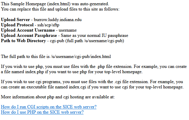
📦 “Real World” Web Sites and “Real World” Web Servers
Starting a “real world” website involves several more steps: (1) obtain a domain name from a domain name broker service, (2) rent or configure a Linux machine with a web server like Apache or nginx, (3) configure the DNS A or AAAA record to resolve to the server’s IP address, and (4) move content into the server’s content folder (e.g. on Apache:
/var/www/html).It’s a misnomer to draw a line between the “real world” and a “fake world”: you’re building real things in this class, so everything you do is part of the real world. But like many abstractions, we gloss over details: such as how
make-cgiis a Perl script maintained by Rob Henderson (SICE IT) that configures a series of extended access control list (ACL) options in order to make a folder stored in a user’s (private) home directory accessible to anyone with an internet connection.
Web Page Foundations
With our cgi-pub directory configured, we’re ready start writing individual web pages to collectively progress toward coherent web sites.
Web pages are made up of three programming languages:
-
HTML: Hypertext Markup Language - a markup language to represent types of content (headers, sections, paragraphs) and the content itself: informing a web browser what to display
-
CSS: Cascading Style Sheets - a domain specific programming language used to style and layout content in a web page: informing a web browser how to display it
-
JS: JavaScript - a general purpose programming language used to make web pages dynamic by responding to a user’s interactions with the page. This language works best alongside HTML and CSS (front end), but JavaScript is also used on the back end to write applications and interact with databases (e.g. Node.js)
Although these three languages work in conjunction, that dance 🪩 is reserved for other courses.
In this course: we focus on writing content in HTML, and we will rely on a front-end framework called Bootstrap that packages CSS and JavaScript into a pre-built component library. This will give us the tools to build a professional-looking website, while leaving some details (how CSS and JS actually work) as future topics.
We’ll get back to the front end in unit 2. For now, let’s focus on writing content.
HTML and the Document Object Model
Hypertext markup language (HTML) is an example of a markup language with a relatively simple structure for both humans and machines to read.
Each HTML tag represents a type of content. Many of these tags are drawn from terminology developed out of the needs that typically arise while publishing written material:
<article>- a discrete composition<section>- a discrete section in an article or document<h1>- the main header, such as a page title<h2>- the secondary header, like a subsection<p>- a paragraph
When HTML is read into a browser, the browser parses (breaks into distinct pieces) the tags into (surprise!) a tree-like data structure consisting of parents and their children. For example, an individual web page for a news article might be structured to contain a <body>, which in turn contains the actual <article>. The article contains a large header (<h1>) at the top, followed by multiple sections which each contain sub-headings (<h2>) and paragraphs (<p>).
<html>
├── <head>
│   ├── <title>
│   └── <link>
└── <body>
    └── <article>
        ├── <h1>
        ├── <section>
        │   ├── <h2>
        │   └── <p>
        └── <section>
            ├── <h2>
            ├── <p>
            └── <p>
Each HTML tag is responsible for two things: the type of the content, and the content itself. For example, in this listing:
<h1>Title Goes Here</h1>
The content type is a level-1 heading <h1>, and the content itself is Title Goes Here.
Without HTML, we just have text:
HTML

HTML HyperText Markup Language (HTML) is the standard markup language for
documents designed to be displayed in a web browser. It defines the
content and structure of web content. It is often assisted by
technologies such as Cascading Style Sheets and scripting languages such
as JavaScript.

-- Wikipedia
… which is informative, but perhaps not the most readable.
It’s best to aim for “semantic” markup, where we use the full range of HTML tags to give the best meaning possible to content. Well marked-up content has several implications for (1) improved accessibility, such as for users with screen readers, (2) achieving better rankings in search engines, (3) providing re-usable components when styling a page, and (this is the “semantic” part) (4) providing context for the content within.
Writing HTML is incremental: content and structure can be separate, so one may focus on one or the other before reaching a result. We might start with the text content above, and structure it with appropriate tags like this:
<h1>HTML</h1>
<p>
<strong>HyperText Markup Language</strong> (<strong>HTML</strong>)
is the standard markup language for documents designed to be
displayed in a web browser. It defines the content and structure of
web content. It is often assisted by technologies such as Cascading
Style Sheets and scripting languages such as JavaScript.
</p>
<p><a href="https://en.wikipedia.org/wiki/HTML">— Wikipedia</a></p>
HTML Reference
Dividers
The most generic tags are for a box (or “division”) for layout and a paragraph for text.
<!-- an empty box -->
<div></div>
<!-- a paragraph -->
<p>Place text here.</p>
Our main focus will be on marking up our content, meaning text, images, links, lists and tabular data.
Keep in mind that although the browser has a default style sheet (CSS) built in, pages marked up with ONLY HTML are not pretty, however the content should have a clear hierarchy and each piece should seem to have a role within the page.
Text
<!-- headlines go up to <h6> -->
<h1>Title</h1>
<h2>Chapter</h2>
<h3>Subhead</h3>
<!-- any text that is not a headline, is a probably a paragraph -->
<p>Text content</p>
Some tags require attributes to provide additional information, link to CSS, or connect to JavaScript. Attributes are ALWAYS written with no spaces as name="" and are separated by a space within the opening tag only.
<p class="byline">By Erika Lee</p>
   ^-- attribute to connect to some CSS for specific styling
It’s possible to have more than one attribute on a tag. It’s also possible to have more than one class on a tag. Classes are how we connect our content to styling declarations within the CSS.
<p class="lead centered" id="introduction">Multiple classes</p>
If multiple classes are present, just separate the class names by a space (as done here with lead and centered). Same with multiple attributes (class and id). Separate by a space, but no spaces within the attribute (i.e. between the name, equals sign and double quotation marks).
Images
Images require the alt attribute. Think of it as a short description for the image.
<!-- images require the alt attribute -->
<img src="images/logo.png" alt="logo">
Links
<!-- links can point to a page in your website -->
<a href="about.html">About</a>
<!-- links can point to another site on the web -->
<a href="https://en.wikipedia.org/wiki/HTML">What is HTML?</a>
Lists
Lists come in two varieties: unordered lists (<ul>) and ordered lists (<ol>). In both cases: each item in the list is a list item (<li>):
|
|
|
|
Tables
Tables are for displaying information in a row and column format.
<table>
    <tr>
        <td>Row 1: Column 1</td>
        <td>Row 1: Column 2</td>
    </tr>
    <tr>
        <td>Row 2: Column 1</td>
        <td>Row 2: Column 2</td>
    </tr>
</table>
Nesting: Tables show us that HTML tags can and usually are nested. Think of each HTML tag as a box being drawn on the screen. Websites are really just a set of nested boxes. Notice that tags DO NOT OVERLAP like <h1><p></h1></p>.
TABLE starts and stops the tabular data section. The TR stands for “table row” and the TD stands for “table data” and represents the column.
Follow Along with the Instructor
Practice with the instructor: command line interfaces, basic HTML, Unix/Linux file systems, and remote servers.
Practice
We’ll build a two page site with just enough CSS to make our content look nice:
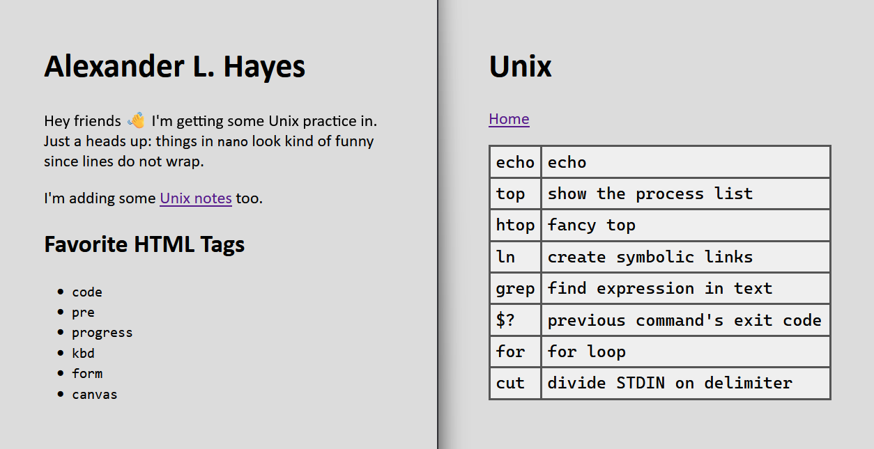
01 Connect to the Remote Server and Setup CGI
Today we’d like you to access the Silo server, provided by Informatics, using ssh:
Open a terminal, then follow along in “Secure Shell Client: ssh” above using your IU credentials (username and password).
TIP: Remember that the password is hidden as you type (you don’t want people looking over your shoulder and knowing your password). It’s okay if it takes a couple attempts.
02 Setup CGI
Once you’re logged in, run the make-cgi command as shown in “Web Sites and Web Server Foundations” above which will create a cgi-pub directory and allow us to run websites and web applications.
03 Set up a basic website structure
- Navigate to
cgi-pub - Using the command line, set up the following basic structure for a web site project:
first-website/
├── unix.html
├── css
│   └── style.css
└── index.html
04 Add HTML content to the home page
Use nano to add the following code for a blank web page to index.html, then save your work.
<!DOCTYPE html>
<html lang="en">
<head>
    <meta charset="UTF-8">
    <title>First Website</title>
    <link rel="stylesheet" href="style.css">
</head>
<body>

</body>
</html>
Inside the body, add:
- a heading with your name
- a paragraph with a welcome message
- a link to
unix.html - a second-level heading labeled “Favorite HTML Tags”
- a list with some of your faves; skip the
< >greater than / less than signs
When you are done, save your file.
View the result in a browser, replacing USERNAME with your IU username:
https://cgi.luddy.indiana.edu/~USERNAME/first-website/
👀 Notice how the directory structure carries over into the URL
The
cgi.luddy.indiana.edu/~USERNAMEpart connects to thecgi-pubdirectory. Anything inside—like thefirst-websitedirectory—becomes part of the URL. We don’t need to addindex.htmlto the end since it’s the default.
05 Add HTML content to another page
Use nano to add the code for a blank web page to unix.html, then save your work.
In the body, add:
- a headline titled “Unix”
- a link called “Home” that goes back to the home page
- a table: two columns, at least 4 rows (Hint: copy-paste our table example)
- for each table row:
- add a unix command to the first column (e.g. pwd)
- add a brief description in the second column (e.g. print working directory)
View the result in a browser, replacing USERNAME with your IU username:
https://cgi.luddy.indiana.edu/~USERNAME/first-website/unix.html
👀 Notice that the file name is now referenced in the URL
Because we are no longer on the default “index.html” page!
06 Test the Links in Your Site
In the browser, do the links between the two pages work?
If not, make sure you are using a relative path—one based on where files are in relation to each other.
Hint: Use relative paths
Since
index.htmlandunix.htmlare in the same directory, we can use the file names directly:<p><a href="unix.html">Unix</a></p>Or we can be precise that the file is in the same directory with
./:<p><a href="./unix.html">Unix</a></p>
07 Add styling using CSS
Navigate to styles.css and add the following:
body {
    background-color: gainsboro;
    font-family: Seravek, 'Gill Sans Nova', Ubuntu, Calibri, 'DejaVu Sans', source-sans-pro, sans-serif;
    font-size: x-large;
    padding: 2.0rem 4.0rem;
}
Save and view the results in the browser.
08 Is the CSS working?
Does the site look how you expected? Is the CSS loading in correctly?
The style.css should be in the css/ directory. How do we adjust the href link to make it load in correctly?
<link rel="stylesheet" href="style.css">
Hint: Relative links!
When a file is in a directory, we must specify the path to that file.
<link rel="stylesheet" href="./css/style.css">
09 Nicer tables
Edit the css/style.css file again, this time adding CSS to make our table of Unix commands look nicer:
table {
    font-family: ui-monospace, 'Cascadia Code', 'Source Code Pro', Menlo, Consolas, 'DejaVu Sans Mono', monospace;
    width: 100%;
    background-color: #efefef;
    border-collapse: collapse;
}

td {
    padding: 0.3em;
    border: 3px solid #555;
    vertical-align: top;
}
Wrapping up
Did any of this feel annoying or like a lot of work? 😡 😤 🤬
We’ll be upgrading our text editor to VS Code soon, and then most of the struggle with file editing will fade away. The goal is to understand what the tools you use are doing for you and to build your workflow (as you learn) to speed up the boring or repetitive parts, without compromising your decision making.
Further Reading
- Neal Stephenson, “In the Beginning… was the Command Line”
Footnotes
“People” on a Linux server is broadly defined. For example: some accounts could be shared between multiple human users, while other accounts are reserved for “bots” that act on behalf of other users. The most common “bot” is the root account, which (if you’re following best practices) is not used directly, but might be invoked in specific situations to change the system: like when an administrator on the server needs to upgrade software or install a new package.
Forges: Git and GitHub
“It is difficult to overstate the importance of version control. I believe that it is as important as the invention of the chalkboard and of the book for multiplying the power of people to create together.”
Foundries and Foundations
We spent the last couple of lessons defining abstract spaces, their benefits, and their limitations.
In the first lesson we saw a first space: our local machine. We generally have complete control over it: meaning that we can install software, create files and folders, and generally have unlimited freedom. Unlimited freedom may come at a cost. Thou are free to choose whether you back up your files—or not. Thou are free to run untrusted code, lose your files to ransomware, and hope that the scammers are true to their word after you liquidate your life savings into cryptocurrency.
In the second lesson we defined a second space: a remote server. These are shared resources: which means that we have to give up some of our absolute freedom in order to work together with others. We must agree on: what programs are installed there, how the directories get structured, how to share finite processing power, who has the authority to make changes, and how to audit and resolve conflicts.
What choice can we make between absolute freedom and shared governance? Infinite points exist between the two extremes. We can parallel these to sociological ideas about human societies and communities. The first place is the home (where each person’s home is their castle)1 and the second place is the workplace. Third places are everything else: book stores, libraries, coffee shops, public parks, national forests, or fisheries.
If you’re building something for other people or with other people, that third space is called a forge or software forge.
Commons, Clubs, Forges, and Knowledge Work
A forge is a repository where people collaborate to create digital goods. In the early Internet: forges were individual websites or email lists. Since bandwidth—the means of transmitting bits over a wire—was limited, forges had to be augmented with existing physical and human infrastructure: such as a postal service that could physically deliver copies of software on discs from one part of the world to another.
But the story didn’t end there. Storage costs dropped, bandwidth got cheaper and faster, processor speeds compounded exponentially. You may have even read the phrase “postal service” and cringed: why would you send a file on a physical compact disc (CD) when you can download it over the network? The world went through a phase transition and the forges themselves became digital.
As of 2024, the term software forge is used synonymously with the term GitHub. This synonym is a lie:2 but it’s a lie predicated on many of the same factors that led to the forges getting digitized.
No single source of truth: git, version control, and skateboards
Remember how we spent the last couple of lessons talking about Linux? Linux isn’t the only thing that Linus Torvalds invented. He also invented a little program called git.
git, or “the stupid content tracker”, was a response to challenges faced in the 1990s and early 2000s when a team of engineers distributed across planet Earth collaborated to build Linux. Software is malleable—hence the soft in software—any person who has a copy of the software’s source code can change it for better or worse: either they know what they’re doing and they make it better, or they don’t know what they are doing and they break the code. But here inlies a question: if everyone has their own copy of the software, and everyone can make changes, which version is correct?
There did (and still does, c. 2024) exist a correct version of Linux—it’s the version that Linus Torvalds says is correct, and it’s the version that he points kernel.org at. But this leads us into more questions. Are all the past versions of Linux incorrect in some way? How do I know that I have the most up-to-date version? What if I discover a problem and fix it in my copy, how do I tell Linus about my fix? If you’re asking these questions, you’ve discovered the idea behind source control or version control.
Side note: Which skateboard is correct? 🛹
“Skateboarding” is a recent enough invention that we can draw a strong analogy between software and skateboarding if all this source control talk feels too abstract.
Skateboarding is an activity. Every skateboarder is a person who owns a skateboard, but if you go to a skate park you are not going to see every person skating the same or even using the same tools. There is a plethora of skateboard designs, equipment, and tweaks.
The “casual skater” may be satisfied with buying a board and using it however the manufacturer intended, but the “expert hobbyist skater” might not be. Becoming an expert in a craft often coincides with a desire to experiment: wanting to change what is in pursuit of what might someday be. What if I sand off the edges? What if I swap the wheels? How much grease is too much grease?
This evolutionary design among experts and hobbyists produces the skateboard—hobbyists learn from and copy one another, forming feedback loops that cause manufacturers to produce new editions based on what people want.
So which skateboard is correct? — Whichever is correct for you.
In plain speak, what are git and GitHub?
The first thing to learn is that git and GitHub are not the same things:
-
Git is an open source version control system—another program on our list of Linux commands. It is primarily used to track changes in source code, make backups of the code, and allow multiple programmers to work on code simultaneously.
-
GitHub is a website where people manage and collaborate on remote git repositories.
Indiana University has an internal GitHub called IU GitHub at https://github.iu.edu/ that is free to use for students. You can log in with your IU credentials.
Follow Along with the Instructor
Today: we’re doing all the practice steps together, so follow along with the video to practice with the instructor. Our goal is to get started with Git and GitHub—both of which will be required to do homework and projects.
Create a scratchspace repository on IU GitHub
The best way to learn is by doing.
- Open https://github.iu.edu
- Choose “New” (looks like a plus icon ➕)
- Create a new repository called “scratchspace”
- Owner: (your username)
- Repository name: scratchspace
- Description: “Practicing with git and GitHub”
- ✅ Public
- ✅ Add a README file
Think about git as a series of snapshots of your files: at any point in time, what did your files look like?
The initial state, or initial commit of the repository might contain a single file called README.md. So the initial commit is a directory with a single file inside:
gitGraph
    commit id: "🎉 Initial commit"
But if you make changes to that README.md and make a commit, then we’ve created a new snapshot of the code:
gitGraph
    commit id: "🎉 Initial commit"
    commit id: "✨ Add a more descriptive title"
Every time we repeat this edit + commit step, we create a new node in a graph: a timeline or git history progressing from the left to the right:
gitGraph
    commit id: "🎉 Initial commit"
    commit id: "✨ Add a more descriptive title"
    commit id: "✏️ Fix typo in README"
This graph of commits—with older commits on the left and newer commits on the right—shows the entire history of a project. Every commit records what the code looked like at a point in time.
Back at the command line: First-time Git setup
We need to adjust some settings before using git.3
Replace yourUsername with your username, and run these in your shell:
git config --global user.name "yourUsername"
git config --global user.email "yourUsername@iu.edu"
Set the default branch name:
git config --global init.defaultBranch main
Set nano as the default editor when writing commit messages:
git config --global core.editor "nano"
Set a default strategy to follow when pulling changes from a remote repository:
git config --global pull.rebase false
Clone a git repository
Version control generalizes the directories and files we talked about previously. Instead of our files and folders being static: version control is a means of keeping track of their state over time.
Let’s clone a copy of our repository from IU GitHub:
git clone https://github.iu.edu/USERNAME/scratchspace.git
When we change into the directory, we should see it contains the same files from GitHub:
$ cd scratchspace/
$ tree .
.
└── README.md
The scratchspace we cloned is a special kind of directory called a git directory: meaning we can run git commands inside of it. How do we know it’s a git directory?
$ ls -a
.git  README.md
We know this is a git directory because there’s a special .git directory inside of it. For the purposes of this book: one should be aware of two things:
- the .git directory exists
- it represents the base of a repository: everything in the same folder as a .git directory is also part of a git repository
Exactly how this folder works is beyond the scope of what we plan to cover. But there are two implications:
- every subdirectory in a repository is also part of that repository, which one might visualize by walking toward the root until one finds a .git directory (alternatively: finding the root—meaning that one is not in a git repository)
- weird things happen if one puts a git repository inside a git repository:


The takeaway is to be mindful of where one clones or otherwise creates repositories.4 A practice that we’ll follow is to have a common directory (e.g. i211/), and put git repositories (starter/, lecture/, project/) inside of it:
i211
├── starter
│   └── .git
├── lecture
│   └── .git
└── project
    └── .git
Plumbing and Porcelain 🚽
Plumbing and porcelain are two metaphors for thinking about abstractions.5 In an abstraction: the plumbing describes how something works on a technical level. The porcelain, by contrast, describes how something works to an end user.
Plumbing vs. porcelain is not necessarily the same as a distinction of complexity or difficulty. The ability to drive a car and the ability to repair a car are related skills, but proficiency in one does not guarantee the other. Driving is a porcelain skill: requiring one to learn how to steer, operate pedals, and actuate signals. But its porcelain nature does not trivialize the skill: driving a car in the United States requires extensive training before receiving a license.
All this to say: we focus on porcelain git. The mechanics describing exactly what the
.gitdirectory is, how git keeps track of changes, or how git communicates with remote repository are details for another course.
Repo status and remotes
The first one we should know about is status, or the git status subcommand, which we can use to check the state of our local repository:
$ git status
On branch main
Your branch is up to date with 'origin/main'.

nothing to commit, working tree clean
Feedback from the status command leads us into some new vocabulary:
- branch
- origin/main
- working tree
A branch is a line of development, and each commit occurs on the main branch by default. The working tree is git’s terminology for the file tree being tracked. In total: the phrase “nothing to commit, working tree clean” means that none of the files have been changed. Clean versus dirty are common metaphors when keeping track of changes: where a clean file is unchanged and a dirty file has been changed—and therefore needs to be inspected.
The origin/main is related to a concept called remotes or remote repositories. For this repository, running git remote -v shows:
$ git remote -v
origin  https://github.iu.edu/USERNAME/scratchspace.git (fetch)
origin  https://github.iu.edu/USERNAME/scratchspace.git (push)
Showing that the source of the information in this local git repository—its origin—is a remote repository on IU GitHub.
The simplest git workflow: add, commit, push
Here’s our first goal: edit code on our local machine, and sync our code to GitHub. This requires three commands:
git add .git commit -m "Message"git push
These three commands are so common that people frequently report seeing them written out on sticky notes or taped to the side of developers’ monitors.6
What happens if we make a new file?
touch file1.txt
Whereas we previously saw “working tree clean”, we now see:
$ git status
On branch main
Untracked files:
  (use "git add <file>..." to include in what will be committed)
        file1.txt

nothing added to commit but untracked files present (use "git add"
to track)
Since file1.txt is new: it is untracked by default. Here inlies a key difference between version control systems like git and cloud backup systems like Dropbox, Google Drive, or Apple iCloud—just because a file is currently inside a git repository does not mean we want to track it. With git, you must opt in to files getting tracked.
The feedback does suggest we can use the git add subcommand to begin tracking this file. If we run git add .:
git add .
… then git status informs us that we’re ready to commit, and the file1.txt changes from red to green:
$ git status
On branch main
Changes to be committed:
  (use "git restore --staged <file>..." to unstage)
        file1.txt
Continuing to respond to feedback: git suggests we’re ready to commit. A commit (sometimes called a snapshot) represents the state of all our files and folders at some point in history. Every commit must have a commit message describing what the change accomplishes. Here our change is pretty simple, so we might say:
git commit -m "Add empty file1.txt"
… which gives us some immediate feedback:
[main a108582] Add empty file1.txt
 1 file changed, 0 insertions(+), 0 deletions(-)
 create mode 100644 file1.txt
… but something is different in the status (orange emphasis is ours):
$ git status
On branch main
Your branch is ahead of 'origin/main' by 1 commit.
  (use "git push" to publish your local commits)

nothing to commit, working tree clean
We said earlier that origin/main represents the version of our code on GitHub. In the same manner where we saw we had to opt-in to adding files to be tracked: this again shows us that we have to opt-in to synchronizing our code with the remote repository on GitHub. This continues the trend where git does not perform any actions until it is commanded to.
$ git push
Enumerating objects: 3, done.
Counting objects: 100% (3/3), done.
Delta compression using up to 4 threads
Compressing objects: 100% (2/2), done.
Writing objects: 100% (2/2), 222 bytes | 74.00 KiB/s, done.
Total 2 (delta 1), reused 0 (delta 0), pack-reused 0
remote: Resolving deltas: 100% (1/1), completed with 1 local object.
To https://github.iu.edu/hayesall/scratchspace.git
   66e5a29..ab2ef11  main -> main
Finally, we’ve made it full circle and the status of our repository is back to a “working tree clean” state:
$ git status
On branch main
nothing to commit, working tree clean
Staging: analyzing the core git loop
The first three subcommands: add, commit, and push are verbs. They are actions performed on files. If we instead take a file-centric view, we could give names for where our changes go each time we run a command. We hinted at the existence of three places: the working tree, the staging area, and the local git database. Each git subcommand relates a file to one of these locations:
graph LR
    A[Working Tree] -->|git add| B[Staging Area];
    B -->|git commit| C[Local Git Database];
    C -->|modify files| A;
Let’s add three more files and reason through how git commands affect the files and where they are in the loop. Assume that we start from a clean working tree similar to where we ended in the previous section:
$ touch file{2,3,4}.txt
$ ls
file1.txt  file2.txt  file3.txt  file4.txt  README.md
Test Yourself: What does status show? Hint: three files, red or green?
$ git status
On branch main
Your branch is up to date with 'origin/main'.

Untracked files:
  (use "git add <file>..." to include in what will be committed)
        file2.txt
        file3.txt
        file4.txt

nothing added to commit but untracked files present (use "git add"
to track)
Let’s add file2.txt to the staging area:
$ git add file2.txt
Test Yourself: What does status show? Hint: where does red become green?
$ git status
On branch main
Your branch is up to date with 'origin/main'.

Changes to be committed:
  (use "git restore --staged <file>..." to unstage)
        new file:   file2.txt

Untracked files:
  (use "git add <file>..." to include in what will be committed)
        file3.txt
        file4.txt
These highlight how the staging area is a place to assemble software before one permanently commits the changes to the project history. If one were building a rocket: it’s better to test and assemble pieces individually before moving the final product outside to the launch pad.
Git operates on the same principle: not everything that goes into building software needs to be permanently tracked. Software development frequently requires nonlinear turns to get correct, and could even pollute the working directory with irrelevant files which only exist to test out a specific idea. Therefore the slow, methodical approach should give one time to consider what changes are relevant and what changes are not.
If we also add file3.txt: two files will be in our staging area, with one being outside the staging area.
$ git add file3.txt
$ git status
On branch main
Your branch is up to date with 'origin/main'.

Changes to be committed:
  (use "git restore --staged <file>..." to unstage)
        new file:   file2.txt
        new file:   file3.txt

Untracked files:
  (use "git add <file>..." to include in what will be committed)
        file4.txt
In git terminology, an upload is a push, a download is a pull, and all changes are local until they are synchronized with a remote. This completes our state machine for the concepts so far:
graph LR
    A[Working Tree] -->|git add| B[Staging Area];
    B -->|git commit| C[Local Git Database];
    C -->|modify files| A;
    C -->|git push| D[Remote Repository];
    D -->|git pull| C;
Versioning file content
Continuing the previous example, we have a version-controlled directory, and its state as of the most-recent commit is a directory with four files:
$ lt some-file-tree
some-file-tree
├── file2.txt
├── file3.txt
├── file4.txt
└── README.md
Let’s add some text to README.md. If the following listing looks too mysterious, you can achieve the same result using nano.7
echo '# Hello World!' > README.md
Previously: every file was blank. Now: we have a README.md with something new. We can query git to find out what the differences are with git diff, which shows us:
$ git diff
diff --git a/README.md b/README.md
index e69de29..cc0be1e 100644
--- a/README.md
+++ b/README.md
@@ -0,0 +1 @@
+# Hello World!
The same plus symbol + from earlier returns here: but what was previously a conventional way to represent changes is now something we can see and interact with.
We haven’t staged or committed our changes yet, so let’s compare what happens when we make even more changes:
echo -e '\nPractice makes perfect.' >> README.md
… then git will tell us we’ve made three additions:
$ git diff
diff --git a/README.md b/README.md
index e69de29..d9b5e51 100644
--- a/README.md
+++ b/README.md
+# Hello World!
+
+Practice makes perfect.
This feels like a good time to make a commit and bring ourselves back to a clean working tree state.
$ git add README.md
$ git commit -m "📝 Add starter notes"
What makes a good commit? 🤔
There isn’t a universal rule satisfying this question. But the inverse is easy: what makes a commit message bad? Imagine you read someone’s commits to find:
- commit
- commit
- it works
- done
… did you infer what these did?
Good commits are discrete units of work. Good commits tend to be verbs, and good commits tend to be atomic—small, but also difficult to divide.
Compare previous four commits with something like these:
- Add add_user function
- Set an index on user email addresses
- Test for valid vs. invalid usernames
- Document limitations of email validation
Which set do you prefer?
Descriptive commits that make small, incremental changes tend to be easier to understand than poorly-worded commits that make huge, sweeping changes. But perhaps you’re working alone and no other human being will ever see your commits: you will eventually have to face your past self. Was your past self helpful? Did your past self write helpful commit messages, or did they leave you a trail of hieroglyphics to decipher?
Releasing Software
Version control so far has been a behind-the-scenes tool. Why should any end user (someone who interacts with an app we build) care about whether we’re following a version control approach at all? Releases (or release versions) are something we will accomplish with tags, following a semantic versioning approach.
You may already have seen semantic versioning without realizing it or without knowing what it meant. Semantic versions (as defined in the Semantic Versioning 2.0.0 specification, is a simple X.Y.Z numbering approach to communicate version parity with users.
Project milestones might correspond to things that end users want: usually features and bug fixes. Each of these can be a commit
Every release is described by three numbers: MAJOR.MINOR.PATCH.
- MAJOR represents major changes, often those that are backwards-incompatible with whatever versions preceded it
- MINOR represents features being added, but have been done in a way that is backwards compatible
- PATCH represents bug fixes
Now that you know what these three numbers mean: test your knowledge on the following:
- A piece of software requires a minimum version of
v1.1.0. You havev1.2.0installed. Is your installed version compatible with the requirements? - You have
v1.5.1installed. Should it generally be safe to upgrade tov1.5.8? - Alexander has Python
v3.11.2installed. Your friend has Pythonv3.9.0installed. Would you expect a Python program that works for your friend to work for Alexander? Why or why not?
With git, a release is created by tagging a commit with git tag. As an example, creating release v1.0.0
git tag -a v1.0.0 -m "Version 1.0.0 Release"
git push -u origin v1.0.0
Sharing versions: git networking and forges
So great: we have a version-controlled directory on our local machine, and it contains every noteworthy change that we’ve ever made. But remember how we started off this whole discussion with lofty ideas about sharing ideas, using a forge, and communicating with others toward the betterment of the commons? This database exists on our local machine, but we haven’t explored a means of uploading or downloading these versions.
The more-complete way is to think of these as a finite state machine. Using git subcommands will move a file between the locations:
graph LR
    A[Working Tree] -->|add| B[Staging Area];
    B -->|commit| C[Local Git Database];
    C -->|push| D[Remote Repository];
    D -->|pull| C;
    D -->|clone| A;
TL;DR git terminology
Version control with git is a deep topic. Since we assume you’re getting started with git, we want you to be comfortable with a core set of terms and operations. The following are a sufficient set of terms and commands to get you started in a single-developer git workflow using tagged releases. When you work on a team: you’ll want to be comfortable with the git branching model, and merge versus rebase strategies. If you go deeper into operations (GitOps or DevOps), you’ll want a working knowledge of the plumbing-porcelain dichotomy. Right now: practice your fundamentals, and layer in more complexity when you are ready.
| staging area |
| commit |
| remote repository |
.git directory |
.gitignore |
git status |
git diff |
git add [file] |
git commit -m [message] |
git remote -v |
git pull |
git push |
git clone [url] |
git tag -a [version] -m [message] |
TL;DR What is our workflow?
- Before we even begin, we must ask: where do we want to work today?
$ cd to/an/i211/repository
- Make sure that our repository is up-to-date.
$ git pull
Already up to date.
This our local and remote repositories are in sync with each other, and we’re ready to start working.
- Open in Visual Studio Code
$ code .Earlier: we said that the dot represents the current folder. So
code .opens the current folder in Visual Studio Code.
- Edit, stage, and make commits as you accomplish tasks
git add [file-name]       # stage
git commit -m "[message]" # commit
git push
Should we
git pushevery time? Maybe! Pushing effectively “backs up” your code to a remote location, so committing and pushing frequently means we’re less likely to suffer a data loss.
- Once we’re confident in our code and we’ve reached a major milestone, we’ll tag the commit with a version number. For example: create
v1.0.0and push the release to GitHub:
git tag -a v1.0.0 -m "Version 1.0.0 Release"
git push -u origin v1.0.0
Conclusion: a distributed, asynchronous, multi-user model of collaboration
Version control in general, and git in particular, are tools that help to solve the questions that we set out with at the beginning of this lesson.
Are all the past versions of the software incorrect in some way? — yes, but we have them in the history if we need to refer back to them.
How do we know we have the most up-to-date copy of something? — we pull.
I fixed a bug in my copy, how do I tell everyone about it? — we commit and push. Technically: we push our copy into a public branch and open a pull request (or merge request) linking back to a maintainer—but that’s a detail we’ll have to explore at some other time. The key idea is that a version control system (VCS) defines a set of primitive operations. In concert, these primitive operations may be combined into a protocol that groups of people use to communicate with one another. The “single developer tagged release workflow” that we described here is one workflow out of many that you may see out there in “the real world”.
flowchart LR

  subgraph "Person 2"
    direction LR
    G[Local Git Database];
  end

  subgraph "Person 1"
    direction LR
    C[Local Git Database];
  end

  C -->|push| D[Remote Repository];
  D -->|pull| C;
  G -->|push| D;
  D -->|pull| G;
We’ve established the three spaces: our home, our workplace, and the commons. In the following lessons, we’ll orchestrate the three into a common workflow: where we write code (Python) on our local machine, push it into a remote version control system (GitHub), and deploy those changes onto a public server that anyone in the world may interact with (Linux).
How much git should I learn?
Git has over a hundred subcommands to handle almost any asynchronous collaboration workflow. This large surface area makes git one of the most-complex programming tools that isn’t itself a programming language.
If we had more time in this class: we would spend time on branching and merging in a git feature branching workflow. But i211 does not spend time in group projects, so features used for multi-developer workflows would have little utility here. However, one of the key reasons to use git and GitHub are for collaboration: so one should pursue collaboration features once they are comfortable with single-user flows.
As a data-driven approach toward which commands or which parts of git to explore: here are Alexander’s Top-30 git subcommands based on frequency of use:
git add
git status
git commit
git push
git switch
git clone
git checkout
git merge
git branch
git log
git remote
git rm
git diff
git mv
git restore
git pull
git reset
git cat-file
git show
git rev-list
git stash
git grep
git submodule
git revert
git cherry-pick
git fetch
git rebase
git blame
git tag
Further Reading
- Scott Chacon and Ben Straub, (2014) “Pro Git: Second Edition”. Also available online: https://git-scm.com/book/en/v2
- Nadia Eghbal, “Working in Public: The Making and Maintenance of Open Source Software” (2020-08-04), Stripe Press. ISBN: 978-0-578-67586-2
- Joshua Gay, “Free Software, Free Society: Selected Essays of Richard M. Stallman” (2002), GNU Press. ISBN: 1-882114-98-1
- Gene Kim, Jez Humble, Patrick Debois, and John Willis, “The DevOps Handbook: How to Create World-Class Agility, Reliability, & Security in Technology Organizations” (2016), IT Revolution. ISBN: 978-1-942788-00-3
- Eric S. Raymond, “The Cathedral and the Bazaar: Musings on Linux and Open Source By An Accidental Revolutionary” (1999), O’Reilly Media, Inc. ISBN: 0-596-00108-8
- Emma Jane Hogbin Westby, “Git for Teams: A User-Centered Approach to Creating Efficient Workflows in Git” (2015-08-17), O’Reilly Media, Inc. ISBN: 978-1-491-91118-1
- Sam Williams, “Free as in Freedom: Richard Stallman’s Crusade for Free Software” (2002), O’Reilly Media, Inc. ISBN: 978-1-449-32464-3
Footnotes
Semayne’s Case (1604-01-01) 5 Coke Rep. 91. See also: Steve Sheppard (editor), “The Selected Writings of Sir Edward Coke” (2005), Liberty Fund, Inc. Carmel, IN 46032-4564, USA.
Every course is limited in what it can cover and what it cannot cover. GitHub is a private company that produces a closed-source forge on an internal version of its own proprietary forge—but despite this sounding like the setup of a logical paradox: GitHub is the largest software forge, and from my (Alexander’s) experience it’s the one that people have heard of even when they know nothing about software. Some other forges in no particular order: GitLab, Bitbucket, SourceForge, Gitea, soft-serve, Kernel.org, Savannah.
Covering the choice of settings we show here is a bit more technical than I (Alexander) want to get into by default. Some are mundane: git config user.email is a matter of bookkeeping, and configures git with the email address that it should write to its internal database. Others, like git config pull.rebase, exist for historical reasons and because different developers use git in different ways—but since its initial release on 2005-04-07 the tool overall has stayed aggressively backwards-compatible to keep the entire ecosystem from fracturing. One is practical: vim is the default text editor in many Linux environments, but nano is beginner-friendly and less prone to causing panic if someone forgets to type a message. Still others, like git config init.defaultBranch main, are social: after George Floyd’s murder many developers re-evaluated earlier naming choices. Master is a word with historical use in trade skills: the master copy, a masterpiece, a master of science degree. But equally present is the word master in a master-slave exploitationship. Devoid of context: which one do you read?
There do exist situations where developers put repositories-inside-repositories: submodules. The git submodule command is outside what we cover, but it provides one way to represent one repository depending on another. Pro Git Chapter 7 covers aspects of this problem.
Scott Chacon and Ben Straub, (2014) “Pro Git: Second Edition”. Chapter 10.1 Git Internals - Plumbing and Porcelain. Online: https://git-scm.com/book/fa/v2/Git-Internals-Plumbing-and-Porcelain
Rachel M. Carmena (2018), “How to teach Git”
The command: echo '# Hello World!' > README.md does several things. echo behaves like a print() statement in other programming languages: it repeats whatever is sent into it. The greater-than sign > is a standard output (STDOUT) redirect, which sends the output of one command somewhere else. In this case, the combination of these can be thought of as sending data into a file.
Python Programming in a UNIX-like Environment
We’ve now explored computers from the perspective of a “power user”—someone who knows the tools of an operating system and can either leverage them or combine them in novel ways to accomplish their goals.
So far the tools we’ve encountered have been purpose-built tools: programs like ls, mkdir, and touch each have a single well-defined purpose. The touch program adjusts timestamps to create new files. The mkdir program creates directories. But the true power of a computer is not its ability to execute purpose-built tools—those have existed for nearly the same amount of time as humans have existed. The true power of a computer is that they are general-purpose tools: a computer is a tool that can be re-purposed, re-tooled, or re-programmed to accomplish any task which can be described by an algorithm, where an algorithm is a discrete set of steps needed to make a decision.
We will use Python (a programming language), which is one such general-purpose tool which we will use to implement algorithms and construct new purpose-built tools. Since our Python programs will inevitably run on a Unix-like operating system, we spend this lesson:
- Starting and stopping programs to familiarze ourselves with the Unix process model
- Writing Python in a REPL (sometimes called interactive mode), then loading and running programs with the Python interpreter (sometimes called batch mode or batch processing)
Follow Along with the Instructor
We’ll talk through some points from the material, talk through steps of the function design recipe, and implement a rock-paper-scissors game that can be played from the command-line.
Starting and Stopping Programs
Every topic from here starts from a terminal.
What happens if we create a new file—perhaps: always_true.py
touch always_true.py
… and add the following code to it?
while True:
    pass
On its own: nothing. But what if we call upon the python3 interpreter to run that code?
$ python3 always_true.py
Is something happening? Is nothing happening? The machine is doing exactly what we told it to do. We asked it to stay inside that loop forever, which it will do until the program crashes (unlikely), our computer shuts off (which includes running out of battery), or we tell our operating system to interrupt the program.
We can send SIGINT, or the interrupt signal, with the ^ Ctrl + C shortcut.1
$ python3 always_true.py
^C
$
Here is what this shows us:
- we can start a program
- we can wait for that program to complete
- if the program does not halt, there is a bigger and more complex program—an operating system—which we can use to stop another program
Analogy: Task Manager and Activity Monitor
Perhaps something on Microsoft® Windows® went poorly for you in the past, so you got out Ol’Reliable: ^ Ctrl + Alt + Delete, click the “Task Manager” button, then “End Task” the misbehaving program.
Those steps form a direct analogue of sending a SIGINT using ^ Ctrl + C in the terminal. The Windows and macOS desktop operating systems are far-removed from the Linux and Unix-like environments we’re working with, but users of those systems share many of the same needs. Eventually something will go wrong, and users will need a tool that stops an erratic behavior.
Whereas Windows Desktop exposes one familiar tool: Task Manager; modern GNU/Linux/Unix operating systems provide at least five:
SIGTERM terminate SIGINT interrupt SIGQUIT quit & (usually) produce a core dump SIGKILL the nuclear option SIGHUP “hang up”, indicating a connection was lost The details of these are out-of-scope here, and you can read about them when you’re working at a low-enough level of abstraction to need them.1
Instead, here are three concepts you can use immediately:
PID,top, andkill.
- a process id (PID) is a number that the operating system assigns to every process
- the
topshows you processes, as well as theirPIDnumberskilltakes a PID and kills the programTaken together, if you search and kill a misbehaving program:
$ top | grep 'python3' 145633 hayesall ... python3 $ kill 145633Then the other terminal running the misbehaving program will report its death:
>>> while True: ... pass ... [1] 145633 terminated python3 $
A programming language is also a program
Prior to this we used simple programs: ls, cd, mkdir, touch. What happens when you type ls into your terminal and hit ↵ Enter?
The ls command should show you some files and directories. Showing nothing just means there are neither files nor directories. But what happens if you type python3 and hit ↵ Enter?
$ python3
Hopefully (assuming Python is installed) you get something similar to:
$ python3
Python 3.10.12 (main, Nov 20 2023, 15:14:05) [GCC 11.4.0] on linux
Type "help", "copyright", "credits" or "license" for more information.
>>>
This is a REPL, an acronym for “Read, Eval, Print, Loop” (read something from the user, evaluate the expression, print the result of that expression, then loop back to the read step). The REPL gives us a place to type bits of Python code, hit ↵ Enter, and somehow that translates into something happening somewhere on our computer. This can be an extremely useful tool in your toolbox when you’re sketching out a new idea.
The humble REPL is the place we begin and it is the place we will return to many times. The REPL shows us a principle that separates simple programs which may be explained in terms of a fixed number of simple operations (print files, create a new file, make a directory), from non-simple programs which strive toward the infinite.
In the next few weeks: we’ll aim our sights toward writing programs that intentionally continue forever, or at least until someone turns them off.
We just learned about ^ Ctrl + C. Can we use that to interrupt a Python REPL?
>>>
KeyboardInterrupt
>>>
KeyboardInterrupt
>>>
Sort of. SIGINT is a signal—it’s a message from us to the program. It is up to the receiver to listen for that message and interpret its meaning. The interpretation of that message depends on where we are: are we in a Python REPL, or a Terminal Shell?
When we’re in a Python REPL, sending SIGINT appears to print the word KeyboardInterrupt and send us back to the read step. Since we can interract with Python via its REPL, there’s another place the interrupt is reserved to help us with:
>>> while True:
... pass
...
^CTraceback (most recent call last):
File "<stdin>", line 1, in <module>
KeyboardInterrupt
>>>
Do you see it? The SIGINT ^C is right there before the Traceback begins.
When in the REPL: • Use
^Cto get back to the REPL prompt • Use^Dto get back to the Terminal prompt
Designing Programs
Programming language are built from five essential components.2
| Variables | store a value for later use. x = 1 |
| Conditionals | choose a behavior based on an observation. if, elif, else |
| Repetition | repeat a procedure until some condition is met. for, while |
| Abstraction | encapsulate a behavior; hide the details. def, class, import |
| Application | invoke an abstraction to return a result. x + 1 |
Every complex program—operating systems, video games, machine learning models, space shuttles—is at some low level of abstraction doing all five of these things. Major innovations happened over the last fifty years that made computers faster, smaller, and more affordable; but the core operation of transforming data is still here.
In “How to Design Programs”, Felleisen et al. define a “systematic program design” approach as the following six steps. When you’re working alone, these can guide you toward a solution. When you’re working with other agents—prompting large language models (LLMs) or asking someone for guidance—these can communicate where your thoughts are and how you organize ideas.
The Function Design Recipe 🥣
The “How to Design Programs” systematic design steps:3
- From Problem Analysis to Data Definitions. Identify the information that must be represented and how it is represented in the chosen programming language. Formulate data definitions and illustrate them with examples.
- Signature, Purpose Statement, Header. State what kind of data the desired function consumes and produces. Formulate a concise answer to the question what the function computes. Define a stub that lives up to the signature.
- Functional Examples. Work through examples that illustrate the function’s purpose.
- Function Template Translate the data definitions into an outline of the function.
- Function Definition. Fill in the gaps in the function template. Exploit the purpose statement and the examples.
- Testing. Articulate the examples as tests and ensure the function passes all. Doing so discovers mistakes. Tests also supplement examples in that they help others read and understand the definition when the need arises—and it will arise for any serious problems.
Rock-Paper-Scissors
Rock-paper-scissors is a schoolyard game played between two opponents. On each round: players secretly decide whether they will choose rock, paper, or scissors; the winner is then decided based upon the narrative that “paper covers rock”, “rock crushes scissors”, and “scissors cuts paper”.
Check GitHub for your username-i211-starter repository, and clone a copy to your local machine. We’ll be using this repository for the next few lessons (replacing USERNAME with your username):
git clone https://github.iu.edu/i211su2024/USERNAME-i211-starter.git
cd into it:
cd USERNAME-i211-starter
and open the folder in Visual Studio Code:
code .
Working in Visual Studio Code
Visual Studio Code (VS Code) is an open source text editor by Microsoft, which will serve as our editor of choice for the remainder of this book. As of the 2023 StackOverflow developer survey, it was one of the most popular editors (or integrated development environments) with 73.71% of developers listing it as their primary editor.4 Our nano skills are still useful—in the same way we said that most computers are servers that lack a graphical desktop: there are far more computers with nano installed than there are with code installed.
However: we will always recommend starting from a Terminal. Once you’re comfortable with where files and folders exist on your operating system—then it will be fine to experiment with some of the higher-level buttons.
Plenty of online tutorials for VS Code already exist—including official ones created by people at Microsoft. The Introductory Videos playlist is a pretty good place to start for something more in-depth. This covers alternative approaches to topics like breakpoint debugging or version control in a slightly different way.
We do strongly recommend spending some time getting comfortable using a text editor like Visual Studio Code. Some of the common operations when writing code include general concepts like “moving around”, “selecting text”, “editing text”, and “managing windows”.
Refer back to the following tables, which list many frequent shortcuts for Windows, Linux, and ChromeOS (macOS: usually substitute ^ Ctrl for ⌘ Cmd). or review keyboard shortcuts directly inside VS Code by opening the command palette with ^ Ctrl + ⇧ Shift + P.
Moving around and selecting generally involves arrow keys or navigation keys:
| Shortcut | Description |
|---|---|
| arrow keys | move cursor up, down, left, right |
| ^ Ctrl + left/right arrow | move cursor one word left/right |
| ^ Ctrl + up/down arrow | scroll up/down |
| PgUp | Scroll up one page |
| PgDown | Scroll down one page |
| ⇧ Shift + arrow | select text |
| ^ Ctrl + ⇧ Shift + left/right | multi-word select |
| ^ Ctrl + A | Select everything in document |
| Home | Start of line |
| End | End of line |
| ⇧ Shift + Home | Select to start of line |
| ⇧ Shift + End | Select to end of line |
| ^ Ctrl + Home | Start of file |
| ^ Ctrl + End | End of file |
General editing such as save, cut, copy, paste, indent, comment, undo, redo:
| Shortcut | Description |
|---|---|
| ^ Ctrl + S | Save file |
| ^ Ctrl + Z | Undo |
| ^ Ctrl + Y | Redo |
| ^ Ctrl + A | Select all |
| ^ Ctrl + C | Copy selection to clipboard |
| ^ Ctrl + X | Cut selection to clipboard |
| ^ Ctrl + V | Paste from clipboard |
| Tab ↹ | Indent selection |
| ⇧ Shift + Tab ↹ | Un-Indent selection |
| ^ Ctrl + / | Comment-out selection |
Tab and window management is helpful as soon as we have more than one document. Be mindful that by the end of this course our projects will have 30+ files:
| Shortcut | Description |
|---|---|
| ^ Ctrl + ⇧ Shift + P | Toggle “command palette” |
| ^ Ctrl + B | Toggle left sidebar |
| ^ Ctrl + ⇧ Shift + E | Open “file explorer” |
| ^ Ctrl + ⇧ Shift + X | Open “extensions menu” |
| ^ Ctrl + ` | Toggle between code and terminal |
| ^ Ctrl + ⇧ Shift+ ` | Open new terminal |
| ^ Ctrl + ⇧ Shift + 5 | Split terminal vertically |
| ^ Ctrl + PgDown | Next terminal |
| ^ Ctrl + PgUp | Previous terminal |
| ^ Ctrl + P | Toggle “quick open” |
| ^ Ctrl + W | Close current tab |
| Alt + 1 (through 9) | Jump to tab 1, 2, 3, … |
| ^ Ctrl + 1 (through 9) | Jump to tab group 1, 2, 3, … |
| ^ Ctrl + Tab ↹ | Next tab |
| ^ Ctrl + ⇧ Shift + Tab ↹ | Previous tab |
| ^ Ctrl + \ | Split editor |
| ⇧ Shift + Alt + 0 | Swap horizontal/vertical layout |
What subset of Python do we need?
Python does a lot—you might review the Python refresher if it’s been a while.
We’ll definitely need the core of the language: variables, conditions (if, elif, else), loops, functions, and function application. But a few built-in functions, input/output handling, and random number generation (import random) will be needed to.
The built-in input() function is a quick way to get information from the user in the middle of program evaluation, and we can use this to solicit what they want to play:
>>> x = input("scissors/paper/rock> ")
scissors/paper/rock> rock
>>> x
'rock'
So that will handle the human player. How would we build an opponent for them to play against? When you have no prior knowledge about the opponent you’re playing against: the best strategy is to behave randomly. Implementing our own random number generator is outside what we want to cover, but the Python standard library includes a module called random to assist with these tasks:
>>> from random import choice
>>> choice(["scissors", "paper", "rock"])
'paper'
>>> choice(["scissors", "paper", "rock"])
'rock'
>>> choice(["scissors", "paper", "rock"])
'paper'
>>> choice(["scissors", "paper", "rock"])
'paper'
Finally, we should program defensively to guard against bad data getting into our system. But if it does, we should provide feedback on how to correct an improper action. Every program in a Linux system has two kinds of output: standard output (STDOUT) and standard error (STDERR).
Python has a built-in print() function. By default, the function sends output to STDOUT5 using sys.stdout. But this can be changed using the sys.stderr file:
>>> from sys import stderr
>>> human_choice = "cannon"
>>> print(f"Unknown value: '{human_choice}'", file=stderr)
Unknown value: 'cannon'
Goal: Implement RPS
Implement a version of Rock-Paper-Scissors. It should:
- Ask the user to choose an option, possibly many times if they have typos. In the event of a problem: send an explanation to STDERR.
- Choose a random action for the computer.
- Display the winner: human or computer?
Starting from rps.py, fill in the gaps with incremental development where you periodically run the code to see how it works:
from random import choice
from sys import stderr
def is_valid(raw: str) -> bool:
pass
def main():
pass
if __name__ == "__main__":
main()
A complete program might behave similar to this:
$ python3 rps.py
(scissors/paper/rock) >>
$ python3 rps.py
(scissors/paper/rock) >> cannon
Unknown: 'cannon', try again
(scissors/paper/rock) >>
$ python3 rps.py
(scissors/paper/rock) >> rock
Computer chose 'paper'
Computer wins!
$
Practice incremental development. If you get stuck inside the program’s execution, recall that you can send the SIGINT to get back to your shell. If you’re uncertain about an internal state of the program: print debugging is a technique where you add “print statements” to give yourself feedback about about some intermediate program state—just remember to delete them when you’re finished.
How did it go?
Easy 😌. Cool!
Hard 😓. That’s okay. Here’s what I want you to do: get a good night’s sleep and try this exercise again tomorrow. You will come back with fresh eyes and the experience you gained last time. Keep doing this everyday until you see parentheses in your dreams.
I didn’t do it 😳. Go back and try again. Seriously. The only way to learn is by doing. If your plan is to read about solutions then copy & paste: you will not pass this course.
The “Soft Skills” of Software: How to make yourself (and anyone who works with you) miserable
So great: I’ll assume you’re reading this because your Rock-Paper-Scissors implementation is working.
We aren’t ready to explore “The Answer” yet. Since this course assumes you’ve already had at least one or more semesters of programming experience: we instead want to reflect on the code we wrote for RPS, and perhaps on all the code that we wrote previously.
So in this section, we’re going to talk about some “red flags” that come up when reading code.
We’ll use a listing like this one to illustrate problems from time to time. Can you spot a few “red flags” in this code? How might you improve it?
# functions:
# -----------------------
# TODO no longer needed, see the version in 'new_stingify_kxt.py'
# Define the list to string function
def list_to_string(input_list):
"""Author: Alexander L. Hayes"""
strd = str(input_list) # Convert to a string
middle = strd[1:-1] # Take the middle elements
# print("--- Line 16")
# print(middle)
for s in middle: # Added by KXT for debugging
print(s)
return middle.replace(", ", " ") # Replace comma with space
# Print the list_to_string
print(list_to_string([1, 2, 3])) # Use [1, 2,3 ] as example
🚩 Comments
Bad advice: “Make sure to add as many comments as possible!”
Advice: Strive to write code that doesn’t need any.
Why? Comments lie, and there are few things more harmful than reading an out-of-date comment; or online commentary that is no longer valid. Do you want to know what doesn’t lie as often? Code that is routinely validated and tested for correctness. There is a flavor of comments that are closer to code, but they’re called docstrings. More on those later.
🚩 Commented-out code
Bad advice: “You Might Need It Later!”
Advice: No you won’t. Delete it.
Why? We spent several lessons talking about version control systems: tools that allow you to store, transmit, and time travel to any point in history. If you actually do need it later: it’s back there in the history. If it’s something important and you’re worried you’ll forget it: the current file is not the right place for that. Learn to take better notes and refer back to them later.
Need an intermediate solution? Create a new file called notes.py and store any code you think you might need later in it. Just like how your parents probably moved all your little kid toys to the basement, waited until you forgot about them, and then donated them (“Oh I don’t know what happened to that honey 🤷🏻♀️”), you’re going to find you probably DON’T need that code. When you’re ready, delete the file. (And shhh don’t tell Erika’s son about his toys.)
🚩 Zero Functions
Bad advice: “Functions: the fewer, the better!”
Advice: If you can name it: make it a function.
“Abstraction” is the fundamental tool of computing. Designing a good abstraction is hard, but here’s the trick: we need to be on the lookout for them, and leave space for when they do appear.
🚩 Write it all in the main
Bad advice: “Just write everything in the main!”
Advice: Writing code “in the main” is useful during rapid prototyping. As you progress: convert your insights into functions.
If you are not familiar with the phrase “in the main”, it’s possible that the concept was not shown to you when you previously learned programming. Contrast the following two programs. This program puts most of its behavior inside of a function called itersum, and all user-facing behavior is defined using a main guard:
def itersum(lst: list[int]):
out: int = 0
for e in lst:
out += e
return out
if __name__ == "__main__":
print(itersum([1, 2, 3]))
itersum function. All relevant inputs and outputs to the program are defined in a main guard which clearly delineates what the inputs and outputs are.By contrast, this program:
# main guard shown here for emphasis. Removing the `if`
# statement and tabbing the code left is nearly identical.
if __name__ == "__main__":
out = 0
lst = [1, 2, 3]
for e in lst:
out += e
print(out)
… makes no clear distinction between inputs and outputs. The input is left implicit, and one must manually trace the full program’s logic to arrive at why some output is the consequence of some input.
Here’s the key point: running both programs produces the same result. The result is objectively the same, but which program is going to be easier to read and extend?
As you develop your development skills, your __main__ sections should grow smaller and smaller. When we’re ready to write Flask servers in a few weeks: our main block will be a single line of code:
if __name__ == "__main__":
app.run()
A possible rock-paper-scissors solution
Many students that I (Alexander) have taught want to know the solution to a problem. So here I must caution you: The solution does not exist. What is presented here is “one possible solution of many”, not the Solution-with-a-capital-S.
Here are some rough steps to help you learn:
- Find a problem
- Try to solve it
- Compare your solution to someone else’s solution
- Identify the differences between the two
- Ask yourself some questions about those differences
- Do you like a choice better?
- Is there some new idea I can use?
Try these five steps with your solution and my solution:
from sys import stderr
from random import choice
def is_valid(raw: str) -> bool:
"""Is the raw input a valid choice?"""
return raw in ("rock", "paper", "scissors")
def beats(this: str, that: str) -> bool:
"""Does `this` beat `that`?"""
return (this, that) in (
("rock", "scissors"),
("paper", "rock"),
("scissors", "paper"),
)
def get_computer_choice() -> str:
"""Choose from (rock, paper, or scissors)"""
return choice(("rock", "paper", "scissors"))
def get_human_choice() -> str:
"""Ask the"""
while True:
if is_valid(human := input("(rock/paper/scissors) >> ")):
break
print(f"Unknown {human}, try again", file=stderr)
return human
def main():
"""Play a full game of rock/paper/scissors"""
human = get_human_choice()
computer = get_computer_choice()
print(f"Computer chose '{computer}'")
if human == computer:
print("It's a tie!")
elif beats(human, computer):
print("Human wins!")
else:
print("Computer wins!")
if __name__ == "__main__":
main()
Step 1 in the Function Design Recipe suggests that we start by identifying the data we need to represent. Our inverted game of rock-paper-scissors needs to represent data about what beats what? Jumping to Steps 5, the beats(this, that) answers whether this beats that:
def beats(this: str, that: str) -> bool:
"""Does `this` beat `that`?"""
return (this, that) in (
("rock", "scissors"),
("paper", "rock"),
("scissors", "paper"),
)
How did we arrive at something like this? By thinking through examples for how we would use such a function (Steps 2-3):
>>> beats("scissors", "rock")
True
>>> beats("paper", "rock")
False
Were there other ways we could have done this? Absolutely! Maybe you find functions to be unnecessary here, and instead chose to encode the core problem of “what beats what” as a chain of if/elif-statements:
if human == computer:
print("It's a tie!")
elif human == "paper" and computer == "rock":
print("Human wins!")
elif human == "scissors" and computer == "paper":
print("Human wins!")
elif human == "scissors" and computer == "rock":
print("Human wins!")
else:
print("Computer wins!")
Is this also a valid solution?
Nope. Can you spot the bug that I left in the chain of if/elif/else statements?
Here’s the point: Alexander has been programming for a while. After writing a few million lines of code, he learned to be suspicious of towers of if-statements: too often they caused his eyes glaze over, or else he’d have to exert mental energy checking every case before deciding the whole was sound.
Next Time
We skipped Step 6: we did not talk about testing our code, or any way to think about correctness.
Further Reading
- Matthias Felleisen, Robert Bruce Findler, Matthew Flatt, and Shriram Krishnamurthi, (2014) “How to Design Programs: An Introduction to Programming and Computing” (Second Edition). The MIT Press.
Footnotes
Termination Signals. Online: https://www.gnu.org/software/libc/manual/html_node/Termination-Signals.html
These five follow from a procedural approach to programming and programming languages. Other paradigms exist which may appear to bend these rules—such as structured query language (SQL), which is an instance of a declarative language. A lambda calculus approach to studying languages would tell you that all computation can actually be done with three rules: definition, abstraction, and application—the astute reader may wonder where concepts like conditions and repetition went? The answer is that those concepts can just as easily be defined in terms of abstraction and application.
From: Felleisen et al. 2014, “How to Design Programs”. Used under the terms of the Creative Commons CC BY-NC-ND license. Online: HTDP, Preface, Systematic Program Design
“2023 Developer Survey”, StackOverflow, (May 2023), https://survey.stackoverflow.co/2023/#integrated-development-environment, (accessed 2024-07-09).
Python 3.12.3 Documentation, “Built-in Functions: print”. accessed: 2024-05-02. Online: https://docs.python.org/3/library/functions.html#print
Refactoring & Testing: The Scientific Method of Software
Today we explore a challenge that we’ll spend the rest of the course touching in some way or another: code is a living, breathing document. The software must remain pliable—soft enough to be extended or repaired. Dead letters have a place: hardware which lacks an ability to change can provide a standard for people to work or design against. But this requires the bugs to be features: the hardware may contradict very real facts about the world, but we are forced to live with them.1
- How do we know anything works in the first place?
- How do we know this version works the same as the previous version?
- How do we safely extend the software without breaking it?
In order to create the new: we need something which can be both safe and principled—a scientific system of work.2
In the previous lesson we reviewed functions as our fundamental unit of abstraction: giving a name to an operation defined purely in terms of its input and its output. In the lesson before that we introduced git as a tool to version and “time travel” to any point in history. Today we will try and answer all three questions by exploring another property of functions: they are amenable to automated testing.
Follow Along with the Instructor
We’ll talk through most of the material from this chapter. Along the way this continues to demonstrate Unix, VS Code, Git, and Python.
From Manual to Automated Testing
Imagine you are tasked with the following:
Create a Python script:
sketching.py. Inside of it, define a function:my_sum(lst: list[int]). This function returns the sum of all integers in the list.>>> my_sum([]) 0 >>> my_sum([1]) 1 >>> my_sum([1, 2, 3]) 6
The function signature and input-output pairs provide enough information to get started, since \(1 + 2 + 3 = 6\). So maybe you mash the keyboard for a few minutes and come up with something like this:
def my_sum(lst: list[int]) -> int:
"""Return the summation of `lst`, like `sum(lst)`"""
out = 0
for x in lst:
out += x
return out
Since you’re following a How to Design Programs to the function design recipe, you manually tested this function in one of two ways.
(1) You added a main block at the end of sketching.py:
if __name__ == "__main__":
print(my_sum([]))
print(my_sum([1]))
print(my_sum([1, 2, 3]))
… meaning that running the script produces something comparable to:
$ python3 sketching.py
0
1
6
(2) Or perhaps you manually tested the function by importing the function from sketching, then interacted with the REPL to see whether input-output pairs were consistent with the instructions:
>>> from sketching import my_sum
>>> my_sum([])
0
>>> my_sum([1])
1
>>> my_sum([1, 2, 3])
6
by passing sample inputs into it and observing whether all of them met your expectations.
>>> my_sum([])
0
>>> my_sum([1])
1
>>> my_sum([1, 2, 3])
6
For both cases (1) and (2), there was an expectation about the expected result of the function, which was verified by running the code.
Here’s an idea: let’s automate this testing process as its own script. If we put testing code in a new Python script, test_sketching.py, every time we run the code we will get near-instant feedback for whether our code behaves the way we expect it to.
$ touch test_sketching.py
We can automate our key ideas with the following: the test script refers to a function in sketching.py, and asserts whether the output of each function is equal to an expected result:
from sketching import my_sum
assert my_sum([]) == 0
assert my_sum([1]) == 1
assert my_sum([1, 2, 3]) == 6
If all of our functions work, then it should look like nothing happens (because every assert succeeded):
$ python3 test_sketching.py
… but if we were to add a failing test, a test that we expect should fail:
from sketching import my_sum
assert my_sum([]) == 0
assert my_sum([1]) == 1
assert my_sum([1, 2, 3]) == 6
+ assert my_sum([2, 2]) == 5
… then then the traceback will confirm our expectation that \(2 + 2\) does not in fact equal 5:
$ python3 test_sketching.py
Traceback (most recent call last):
File "~/hayesall/test_sketching.py", line 6, in <module>
assert my_sum([2, 2]) == 5
AssertionError
This example demonstrates the key concepts behind unit testing. In unit testing, one isolates parts of the whole source code into discrete units of expected behavior, often at the level of functions. Those units are tested with more code: functions that answer whether other functions are behaving as expected.
Notice we use the term “expected behavior”, and not “correct behavior”. Running unit tests can answer whether outputs match: not whether the unit tests are correct in the first place. “Correctness” is a mathematical fact requiring proof (by induction, by contradiction, etc.), and a finite list of facts does not guarantee correctness when an input space is infinite. But mathematical correctness is rarely the goal: code is designed to model things which occur in the world, and many things in the world have fuzzy edges which lack clear definitions.
But despite what may seem like surface-level weaknesses: unit testing has shown itself to be sufficient at handling the questions we started with:
-
How do we know anything works in the first place? - we enumerated our expectations in code: if the tests pass, then it probably works
-
How do we know this version works the same as the previous version? - we ask whether the tests still pass
-
How do we safely extend the software without breaking it? - we monitor the state of our tests over time, and avoid making changes that break our tests
(🦉) Build your own testing framework
Draw the owl. Intermediate or advanced students may be interested drawing the owl here for a transparent view into how testing works—or this can remain opaque and one can skip directly to unit testing usage in Python.
Many programming languages build unit testing into the standard library—in Python this is the unittest library—or recommend to implement testing using third-party libraries. Before jumping into “How to use unit testing”, we’ll offer a chance to “Build your own testing framework” using only the core language.
(🦉) Setting a goal
There are two stakeholders: (A) people who write tests, and (B) people who run the tests. Group (B) is likely interested in questions like: did everything work? what didn’t work? where is the problem? did a change break the test? The needs of group (A) must be contended with, but the “usability” of a unit testing framework is something we’ll ponder when actually writing the code.
We’ll meet their needs with a text user interface, perhaps like the output shown in the following listing. From this outside view of how the program works—we see that it shows some statistics about how many tests passed, failed, or raised an exception; then it isolates a specific test that failed—how might you implement this?
$ python3 test_sketching.py
3/4 passed
1/4 failed
0/4 raised
failed: my_sum([]) == 1, got: 0
Answer the following questions; most will be discussed in the text itself.
- Question 1: Starting from the function design recipe, what is the essential data being represented in this problem?
- Question 2: What is the difference between a passed test, a failed test, and a test which raised an exception? Why might one be interested in each of these?
- Question 3: Write a function signature to take the data from question 1 and produce output statistics.
- Question 4: Write a function signature taking output statistics and “visualize” it as a string: the output in the text user interface.
- Question 5: What information is left out of this listing? Is this interface better or worse than the traceback created when running the
assertstatements?
(🦉) Problem analysis and data representation
Recalling step 1 in the function design recipe, we showed that the key information when testing was: (1) the function being tested, (2) its input, and (3) the expected output.
We already showed that we could represent the three needs using assert statements, function calls, and an equal check == in a separate test_sketching.py script:
# file: test_sketching.py
from sketching import my_sum
assert my_sum([]) == 0
assert my_sum([1]) == 1
assert my_sum([1, 2, 3]) == 6
But testing our code like this has limitations. What would happen if we added a failing test above every other tests?
from sketching import my_sum
+ assert my_sum([]) == 1
assert my_sum([]) == 0
assert my_sum([1]) == 1
assert my_sum([1, 2, 3]) == 6
When Python interprets code from the top of a file to the bottom, so it will stop executing immediately when it encounters a problem. So even if 75% of the tests would have passed, we are left with a binary observation: “it works or it does not work”. A helpful interface into this problem could be to (1) run every test, (2) compute some statistics, and (3) help the tester isolate where a problem is.
In order to compute statistics and run every function, we need to represent them in a data structure. Since we have a series of functions and their output, let’s start representing the data as a list of tuples list[tuple[...]]. Specifically: the first value in this tuple will be the function (with input) being tested, and the second will be the expected output. Being more precise, the first is a function (a Callable), and the second can be anything (Any type):
from sketching import my_sum
tests = [
(my_sum([]), 1),
(my_sum([]), 0),
(my_sum([1]), 1),
(my_sum([1, 2, 3]), 6),
]
But just a moment, there’s something subtly wrong with our list of tests. Perhaps Guido van Rossum didn’t read Friedman and Wise3 before inventing Python. When we define a list of tests as a list containing tuples containing function calls, every call is evaluated immediately when the list is created.
>>> from test_sketching import tests
>>> tests
[(0, 1), (0, 0), (1, 1), (6, 6)]
Because of this: we lose information. When we look at the tests list, it’s unknowable what function is being tested and what input resulted in each output. But there’s a fairly straightforward fix for our data structure: separate the name of each function from a tuple containing its arguments and the expected output:
tests = [
(my_sum, ([],), 1),
(my_sum, ([],), 0),
(my_sum, ([1],), 1),
(my_sum, ([1, 2, 3],), 6),
]
… meaning the tests list now preserves the distinction between a function and its input. A function signature that uses this data will handle tuples containing a Callable, a tuple of unknown size tuple[Any, ...], and any output depending on what the function returns Any.
>>> tests
[(<function my_sum at 0x7f2f1b8a9990>, ([],), 1),
(<function my_sum at 0x7f2f1b8a9990>, ([],), 0),
(<function my_sum at 0x7f2f1b8a9990>, ([1],), 1),
(<function my_sum at 0x7f2f1b8a9990>, ([1, 2, 3],), 6)]
(🦉) Implement the tester
Now that we have a list of tests we can implement a function that takes this list of tests; iterates through them while unpacking the function, its arguments, and its expected value; then performs evaluation to check whether expectations are met:
from typing import Any, Callable
from sys import stderr
# ...
def run_tests(tests: list[tuple[Callable, tuple[Any, ...], Any]]) -> None:
for (func, args, expect) in tests:
if (reality := func(*args)) != expect:
print(f"expected {expect}, got {reality}", file=stderr)
if __name__ == "__main__":
run_tests(tests)
For now we’ve only printed the case where the expected output was not the same as the actual output:
$ python3 test_sketching.py
expected 1, got 0
This informs us that one of the tests failed, but does not tell us which function nor which arguments caused the failure. We’ll remedy this by creating a string showing what was tried and what the result was:
for (func, args, expect) in tests:
if (reality := func(*args)) != expect:
- print(f"expected {expect}, got {reality}", file=stderr)
+ argstr = ",".join(map(str, args))
+ call = f"{func.__name__}({argstr}) == {expect}"
+ print(f"failed: {call}, got: {reality}", file=stderr)
$ python3 test_sketching.py
failed: my_sum([]) == 1, got: 0
Since everything that does not fail passes, then we can visually inspect the results to see that one test failed, and the remaining three passed:
for (func, args, expect) in tests:
if (reality := func(*args)) != expect:
# ...
+ else:
+ print("passed", file=stderr)
$ python3 test_sketching.py
failed: my_sum([]) == 1, got: 0
passed
passed
passed
(🦉) Test statistics and output handling
We’re 90% of the way to our goal since we can visually inspect the output to arrive at the solution we wanted. The final step is therefore a matter of output formatting. Instead of printing one output per line, let’s incorporate a new data data structure where we can accumulate intermediate information to while the for loop runs:
result = {"passed": 0, "failed": 0, "messages": []}
In plain speak, the result we’re interested is the statistics for how many tests passed, failed, and a set of messages to inform the user which tests were problematic. With the dictionary initialized at the start of the function, all that remains is to update it inside the function by incrementing incrementing one of the numbers, or appending failure messages. Finally, we will compute the total number of tests as the sum of passed tests and failed tests, and show all of the messages:
def run_tests(
tests: list[tuple[Callable, tuple[Any, ...], Any]]
) -> None:
result = {"passed": 0, "failed": 0, "messages": []}
for func, args, expect in tests:
if (reality := func(*args)) != expect:
argstr = ",".join(map(str, args))
call = f"{func.__name__}({argstr}) == {expect}"
message = f"failed: {call}, got: {reality}"
result["failed"] += 1
result["messages"].append(message)
else:
result["passed"] += 1
total = result["passed"] + result["failed"]
print(f"{result['passed']}/{total} passed", file=stderr)
print(f"{result['failed']}/{total} failed", file=stderr)
print("\n".join(result["messages"]), file=stderr)
$ python3 test_sketching.py
3/4 passed
1/4 failed
failed: my_sum([]) == 1, got: 0
(🦉) Exercises
Notice the previous output was not exactly like the goal we set out with yet. We suggested, but did not handle, the fact that Python raises Exceptions as its primary error handling mechanism. We leave this observation as an exercise (it’s not as important how to get the error handling right, but trying to get the error handling leads to interesting corner cases that we’d like the interested reader to explore).
$ python3 test_sketching.py
3/4 passed
1/4 failed
- 0/4 raised
failed: my_sum([]) == 1, got: 0
We recommend exploring two directions: error handling while testing, and communicating tests to an end user.
- Exercise 1: As written,
run_tests()has multiple responsibilities: running tests and printing results. Design a separate function responsible for output handling. What are thatexplain()functions inputs? What shouldrun_tests()return to make this viable? - Exercise 2: Read about
jsonencoding and decoding in the Python standard library documentation. Write a function to serialize theresultdictionary to a JSON file. - Exercise 3: JSON is a common “interchange” format to communicate data between programming languages, particularly on the web—JSON actually stands for “JavaScript Object Notation”. Write an HTML page visualizing contents in the JSON file.
- Exercise 4: What currently happens in our
run_tests()implementation when a function raises an exception? (e.g. if there is araise ValueErrorinside ofmy_sum())? - Exercise 5: Adapt the
run_tests()implementation to catch exceptions instead of crashing. Represent this with one more test output type: passed, failed, and raised. - Exercise 6: What if we expect a function to raise an Exception? How would you adapt the expected outputs to handle this case? How would you communicate those to the user?
- Exercise 7: What if we don’t expect a function to raise an Exception, but it does? How would you adapt
run_tests()to handle this case?
Python testing with unittest
The Python standard library contains a unittest module. This module contains common fixtures to define groups of test cases, and the necessary function to run tests.
The convention is that testing scripts are prefixed with test_, and contain:
# test_sketching.py
import unittest
from sketching import my_sum
class TestSummation(unittest.TestCase):
def test_empty_list_is_zero(self):
self.assertEqual(my_sum([]), 0)
if __name__ == "__main__":
unittest.main()
Using a class is incidental to this exercise: you don’t really need to understand what a “class” is to infer what this code is doing.4 Nevertheless, we should see a few examples and practice. Let’s start remove some of the details to arrive at a listing to use as a template for testing code:
import unittest
import __________
class __________(unittest.TestCase):
def __________(self):
self.assertEqual(__________, __________)
if __name__ == "__main__":
unittest.main()
The four questions of unit testing
We can fill-in-the blanks through asking a series of questions.
Question 1: What module are we testing? Our tests are inside the test_sketching.py script, and we want to test sketching.py, so we first need to import the module that is relevant to our goal:
import unittest
+ import sketching
class __________(unittest.TestCase):
def __________(self):
self.assertEqual(__________, __________)
if __name__ == "__main__":
unittest.main()
Question 2: What fact do we want to assert? We previously wrote a series of assert statements, like my_sum([1]) == 1. We can fill in the next two blanks using the input and output from this assertion:
class __________(unittest.TestCase):
def __________(self):
+ self.assertEqual(sketching.my_sum([1]), 1)
Question 3: In English, what fact are we asserting? Function names are typically verbs, and we’re writing a function that tests whether the result of calling some function is equal to something else. In this simple example, we “test summing 1 is 1”. Perhaps this seems trivial here, but the benefit of plain-English names pays off when we test more complex behaviors (e.g. “test user interface contains menu”).
class __________(unittest.TestCase):
+ def test_summing_1_is_1(self):
self.assertEqual(sketching.my_sum([1]), 1)
Question 4: What group of behaviors are we testing? Usually there is a logical grouping to our tests, called a TestCase. Earlier we had multiple input-output pairs that tested whether our my_sum function met expectations, so collectively we might call this a:
+ class SummationTest(unittest.TestCase):
def test_summing_1_is_1(self):
self.assertEqual(sketching.my_sum([1]), 1)
Putting the pieces together: With these four questions answered, we have a complete unit testing script, and can convert our remaining assertions into functions:
import unittest
import sketching
class SummationTest(unittest.TestCase):
def test_summing_1_is_1(self):
self.assertEqual(sketching.my_sum([1]), 1)
def test_summing_empty_is_0(self):
self.assertEqual(sketching.my_sum([]), 0)
def test_summing_1_2_3_is_6(self):
self.assertEqual(sketching.my_sum([1, 2, 3]), 6)
if __name__ == "__main__":
unittest.main()
Running unit tests and observing behavior
Running this script from the command line now informs us that all of our tests pass:
$ python3 test_sketching.py
...
---------------------
Ran 3 tests in 0.000s
OK
Each period or dot in this context represents the result of running one of our tests. All three unit tests passed. If we repeat the approach from earlier where we intentionally add a failing test, running the tests will inform us of the existence of a failed test (indicated not with a . but with an F), and return a traceback of the problem:
$ python3 test_sketching.py
..F.
=====================
FAIL: test_summing_2_2_is_5 (__main__.SummationTest)
---------------------
Traceback (most recent call last):
File "~/hayesall/test_sketching.py", line 16, in test_summing_2_2_is_5
self.assertEqual(sketching.my_sum([2, 2]), 5)
AssertionError: 4 != 5
---------------------
Ran 4 tests in 0.002s
FAILED (failures=1)
Here we expected the test to fail and only included it as a demonstration for what the error looked like. Normally we’ll avoid intentionally adding failing tests like this, or if there is some important aspect about it, we might assert a negative case: assertNotEqual(4, 5).
An evolving world + test-driven development
Imagine that something changed out in the world, and now there’s a new behavior that the my_sum function needs to handle:
>>> my_sum(None)
0
Since we already have the code and the unit tests, we might follow a test-driven development workflow. In this workflow, we rearrange steps from the function design recipe and write a test before we attempt to implement the behavior.
# ...
class SummationTest(unittest.TestCase):
# ...
def test_summing_None_is_0(self):
self.assertEqual(sketching.my_sum(None), 0)
# ...
Now: we only consider the code to be complete when the tests pass again. Running the tests reveals our previous code raises a TypeError instead of returning the expected result:
$ python3 test_sketching.py
..E.
=====================
ERROR: test_summing_None_is_0 (__main__.SummationTest)
---------------------
Traceback (most recent call last):
File "~/hayesall/test_sketching.py", line 16, in test_summing_None_is_0
self.assertEqual(sketching.my_sum(None), 0)
File "~/hayesall/sketching.py", line 4, in my_sum
for x in lst:
TypeError: 'NoneType' object is not iterable
---------------------
Ran 4 tests in 0.003s
FAILED (errors=1)
The traceback directs us to a problem in line 4, and informs us that None is not iterable, so the lst variable cannot be None by the time we start the for loop:
def my_sum(lst: list[int]) -> int:
"""Return the summation of `lst`, like `sum(lst)`"""
out = 0
for x in lst: # <---- `for x in None`
out += x
return out
One fix might be to handle this as a special case with an if-statement: returning 0 immediately if lst is None and thereby never reaching the loop:
def my_sum(lst: list[int] | None) -> int:
"""Return the summation of `lst`, like `sum(lst)`"""
if lst is None:
return 0
out = 0
for x in lst:
out += x
return out
… which brings us back to a passing state where all the tests succeed:
$ python3 test_sketching.py
....
---------------------
Ran 4 tests in 0.001s
OK
Refactoring
Martin Fowler and Kent Beck defined refactoring as either a noun: “a change made to the internal structure of software to make it easier to understand and cheaper to modify without changing its observable behavior”, or as a verb: “to restructure software by applying a series of refactorings without changing its observable behavior.”5
We bring up refactoring because its definition relies on testing, or at a minimum: a means of validating behavior in order to be confident that any changes made do not break backwards compatibility.
In the specific case of my_sum, we might refactor into a recursive solution that passes all our tests using half the number of lines of code:
def my_sum(lst: list[int] | None) -> int:
"""Return the summation of `lst`, like `sum(lst)`"""
if not lst:
return 0
return lst[0] + my_sum(lst[1:])
We also bring up refactoring because it emphasizes something about programming that you may not have encountered in an introductory course: programming is hard, but maintenance is harder. As we progress through this course: we will write code, but we will also have to contend with the burden created by the code we wrote earlier.
Documenting, testing, refactoring, and version controlling are each methodologies that evolved in response to the challenges people faced when they tried to maintain code bases with millions of lines. We will see a fraction of these as we progress in this class toward our final project.
Practice: unittest in rock-paper-scissors
We ended our last lesson with questions like: “How do we know if our imlementation actually works?”, or “Should we write a function or not?”. But we didn’t have the right intellectual tools to answer these questions. Let’s explore these using our new unit testing framework, starting with the is_valid(raw: str) -> bool predicate.
def is_valid(raw: str) -> bool:
"""Is the raw input a valid choice?"""
return raw in ("rock", "paper", "scissors")
01 Prepare to work
Start from the same directory where you previously cloned your i211-starter repository.
For example, Alexander would open a new terminal session, change directory into their hayesall-i211-starter directory, then open the folder in VS Code:
$ cd i211su2024/hayesall-i211-starter
$ ls
README.md rps.py test_rps.py
$ code .
02 Run the tests
In the same directory as the rps.py script: there should also be a test_rps.py script. Let’s establish a baseline by running the tests.
How do you run the tests?
Possible Solution
$ python3 test_rps.py . -------------------- Ran 1 test in 0.000s OK
03 Validate that rock is a valid input
Our is_valid predicate returned True or False depending on whether a string entered by the user was a valid rock-paper-scissors choice:
>>> import rps
>>> rps.is_valid("rock")
True
… therefore we might automatically test this behavior with a unit test asserting that we believe "rock" should be a valid choice. Edit your test_rps.py to look like this, and run the tests again:
from unittest import TestCase
from unittest import main as unittest_main
import rps
class ValidateHumanInputs(TestCase):
def test_rock_is_a_valid_input(self):
self.assertTrue(rps.is_valid("rock"))
if __name__ == "__main__":
unittest_main()
04 Validate scissors and paper
Let’s write two more tests to handle the "paper" and "scissors" cases. How would you fill in the blanks in the following listing?
# ...
class ValidateHumanInputs(TestCase):
def test_rock_is_a_valid_input(self):
self.assertTrue(rps.is_valid("rock"))
def __________________________(self):
self.assertTrue(____________________)
def __________________________(self):
self.assertTrue(____________________)
# ...
Possible solution
# ... class ValidateHumanInputs(TestCase): def test_rock_is_a_valid_input(self): self.assertTrue(rps.is_valid("rock")) def test_paper_is_a_valid_input(self): self.assertTrue(rps.is_valid("paper")) def test_scissors_is_a_valid_input(self): self.assertTrue(rps.is_valid("scissors")) # ...
$ python3 test_rps.py
.
--------------------
Ran 3 test in 0.000s
OK
05 Stage and commit
We’ve reached a point where we have working, tested code. Since we’ve accomplished something, this is a good time to make a commit.
How do you make a commit?
Possible solution
git add test_rps.py git commit -m "✅ Add tests for is_valid"
06 How would you test the computer choice?
Our possible RPS solution put the computer behavior into a get_computer_choice() function:
def get_computer_choice() -> str:
"""Choose from (rock, paper, or scissors)"""
return choice(("rock", "paper", "scissors"))
This function does not take an input, but it does produce an output.
What are the expected behaviors, and how might you test those behaviors are true?
class ValidateComputerBehavior(TestCase):
def __________________________(self):
self.assertTrue(____________________)
Possible solution
There are three possible outputs. Even though the behavior is random: we can check that the output is one of the three expected outputs. This parallels a style called property-based testing, where we are not as interested in a specific output, but rather in some attributes or properties of those outputs, such as being one of three choices:
class ValidateComputerBehavior(TestCase): def test_computer_choice_in_rps(self): self.assertTrue(rps.get_computer_choice() in ("rock", "paper", "scissors"))
Alternate solution
Our computer player behaves randomly, which we may want to be mindful of when we test.
If we only run the
get_computer_behavior()function once: then each time the tests run, it may effectively be testing different execution paths through our code. This can be problematic, leading to flaky tests: tests which might sometimes work and sometimes fail.But here, there’s a relatively simple solution: run the tests multiple times. Choosing 10 is arbitrary here: but we might loop over multiple iterations, testing that the computer choice chooses something valid all 10 times:
class ValidateComputerBehavior(TestCase): def test_computer_choice_in_rps(self): for _ in range(10): self.assertIn( rps.get_computer_choice(), ("rock", "paper", "scissors") )
07 Run the tests and commit
If our tests pass:
$ python3 test_rps.py
....
--------------------
Ran 4 test in 0.000s
OK
We’ve accomplished something: making it a good time to stage and commit our changes.
How do you commit?
git add test_rps.py git commit -m "✅ Add tests for computer choice"
08 How would you test that rock beats scissors?
We showed in our possible RPS solution that the core X-beats-Y behavior could be placed in a beats(this, that) function:
def beats(this: str, that: str) -> bool:
"""Does `this` beat `that`?"""
return (this, that) in (
("rock", "scissors"),
("paper", "rock"),
("scissors", "paper"),
)
Test this function (a TestCase class with three methods), run those tests, then stage and commit the changes.
Possible solution
class ValidateWinningCombination(TestCase): def test_rock_beats_scissors(self): self.assertTrue(rps.beats("rock", "scissors")) def test_scissors_beats_paper(self): self.assertTrue(rps.beats("scissors", "paper")) def test_paper_beats_rock(self): self.assertTrue(rps.beats("paper", "rock"))
09 Push and Release
We now have an initial implementation with tests for the core behaviors. This is a good time to create a release which we can iterate on later.
We should:
- push changes to GitHub
- tag a v0.1.0 release of our code
- push the release to GitHub.
What git subcommand steps do we need to accomplish this goal?
Possible solution
Push the main branch:
git pushTag the main branch at v0.1.0:
git tag -a v0.1.0 -m "Initial RPS release with implementation and unit tests"Push the release to GitHub:
git push origin v0.1.0
Further Reading
- Martin Fowler and Kent Beck (2018) “Refactoring: Improving the Design of Existing Code”. Second Edition. Addison-Wesley.
- Gene Kim, Jez Humble, Patrick Debois, and John Willis, “The DevOps Handbook: How to Create World-Class Agility, Reliability, & Security in Technology Organizations” (2016), IT Revolution. ISBN: 978-1-942788-00-3
Footnotes
Was the year 1900 a leap year? Microsoft® Excel® is the poster child of this problem. It mimics the look and feel of tools that came from of a long history of tabulating, accounting, bookkeeping, and data management—the spreadsheet. These tools may be as old as writing itself—the oldest human writings that we know about are tax records and accounting records—so surely it’s easy to produce a facimile of tools which are 12,000 year old? Maybe not. A bug from another spreadsheet program was considered so critical to business operations that almost every version of Excel that has ever existed will incorrectly inform users that 1900 is a leap year.6 Excel and programs based on it are modeled on a world that never existed, and people use it to inform high-stakes decisions: leaving the year 1900 in a kind of Shrödinger box state where it both is and is not a leap year. So the real question is: are people who use the tool knowledgeable enough about these (and similar) shortcomings to prevent catastrophe? Or is there sufficient testing in place to catch the problems when they do occur? Probably not. One does not need to look far before one finds stories on how misuse of Excel is the culprit behind losing critical COVID-19 data.7
To be scientific is to follow in a Newtonian or Bayesian tradition: to develop and participate in a system where we form a guess (hypothesis) about the state of the world, change something, measure it, update our beliefs based on the intervention, then integrate those beliefs into what is already known. This is not to be confused with the goings-ons of scientists, many of whom are least professional, least scientific people out there.8
Daniel P. Friedman and David S. Wise, “Cons Should Not Evaluate Its Arguments”. Online: https://legacy.cs.indiana.edu/ftp/techreports/TR44.pdf
But you, dear reader of footnotes, are obviously curious to learn more. The clear inspiration for Python’s unittest standard library was Java’s JUnit framework—which many people used around the same time that ideas about unit testing were growing more mainstream. Unit testing grew popular around the time that object-oriented design patterns grew popular—if one wanted to go a step further, one might even conclude that object-oriented programming paradigms caused many of the problems that required unit testing to solve.
Martin Fowler (2004-09-01) “Definition of Refactoring”. Online: https://martinfowler.com/bliki/DefinitionOfRefactoring.html
Microsoft, “Excel incorrectly assumes that the year 1900 is a leap year”. Microsoft Learn, Microsoft 365 Troubleshooting. accessed: 2024-05-02. Online: https://learn.microsoft.com/en-us/office/troubleshoot/excel/wrongly-assumes-1900-is-leap-year
Leo Kelion (2020-10-05), “Excel: Why using Microsoft’s tool caused Covid-19 results to be lost”, British Broadcasting Service (BBC), accessed: 2024-05-02. Online: https://www.bbc.com/news/technology-54423988
Richard McElreath, “Science as Amateur Software Development.” https://www.youtube.com/watch?v=zwRdO9_GGhY
Files, Mutable State, and Resources
The most contentious topic in programming is state, or rather how program state should be managed by the programmer(s). The state of a program is the sum total of all a program’s input data and all of the code acting upon that data. When the state is fixed and unchanging, such as with a variable is defined and never updated: we say that the state of a variable is immutable. By contrast, if an object in the language may be updated, we say that the programmer mutated the state of objects in the program.
Programming languages are typically organized in terms of the programming paradigm they inherit ideas from. One of the key ways to distinguish one programming paradigm from another is by analyzing how state gets managed in languages based on that paradigm. In a functional paradigm (C211, C311), state is minimized or eliminated entirely—states do not change, but rather are copied. Java is the quintessential object-oriented language (I311), where state is managed through a tree-structured hierarchy of objects and a rule set defined to answer how state changes and who has permission to change it. In a declarative language paradigm, the programmer describes the states, or describes what they want to occur—and the language “figures out” how to apply those changes (e.g. I308, or later this semester when we discuss SQL).
The Python language is multi-paradigm—implementing aspects of object-oriented and functional paradigms. But many of the concepts we’ve encountered (variables, objects, data types, object attributes, methods) come out of an object-oriented programming interpretation of the language: where the language is organized in terms of objects and methods that modify those objects. We’re also running Python on a Unix-like operating system: which is itself a giant blob of mutable disk space. When Python interacts with the operating system—including when a program reads files or writes to files—we’re inherently dealing with state.
Follow Along with the Instructor
We’ll cover some of the early points in this chapter up to the section on pure versus impure functions. Follow along for some highlights, then work through practice problems when you’re ready:
Stateless Programs
Many of the programs we’ve written up to this point have been stateless. In a stateless program: one can perfectly reason about how the program will behave since all behavior is defined inside the program itself. For example, if we create a new file for a Python script:
touch hello.py
… and add:
print("Hello World!")
How likely is it that when we run the program, we see the word "fish" printed to the console? The probability is low; so low that we might as well conclude that it is impossible. But we shouldn’t be surprised when running the program prints "Hello World!":
$ python3 hello.py
Hello World!
We know this because there is not a dependency in our program on some external data: there is no external information entering our program. No matter how many times we run this program, it should always produce exactly the same result. Let’s draw this as a graph:
graph TB
hello.py
Since stateless programs have no dependencies, using them implies several strengths. They are:
- Easy to reason about. When all the facts are available, one can induce the outputs from the inputs.
- Easy to test. Since stateless programs have clear inputs and outputs, it is usually straightforward to define key behaviors and write unit tests for that behavior.
But stateless programs also come with a huge limitation: since everything is defined up front, they cannot react to anything. The only way for new data to enter a stateless program is by modifying the program. Nevertheless, these can be powerful (well-tested and easily understood) “building blocks” from which we can develop more complex programs from.
Stateful Programs: Randomness
The first narrow form of statefulness we saw was when we wrote programs that included random behavior, usually using Python’s random standard library:
import random
print(random.choice(("A", "B")))
Contrast this program with the “Hello World” program. When you run these two programs, are you certain about the outcome of one but uncertain about the other?
What makes us certain about the outcome of print, but uncertain about the outcome of random.choice? The answer is that the former was stateless, but this one is stateful (more on why in a bit). First let’s clarify something else: we could be uncertain about the random program because its behavior depends on something that we do not control: how random actually works. We can represent this dependency as an arrow (or edge) in a graph and say that the behavior of random_choice.py has a dependency on something inside of random:
graph TB
hello.py
random --> random_choice.py
Now let’s get more precise: Python’s random library is not actually random—its documentation is titled “Generate pseudo-random numbers”. The exact nature of random versus pseudo-random in computing is a story for another time, so for now we will elide the details and focus on this concept: Python has a pseudo-random number generator (PRNG) that produces numbers which are good enough to be used as if they were random.1 A PRNG is based on a seed value determining how the PRNG generates new numbers. Given a particular seed, behavior is deterministic.
import random
random.seed(54321)
print(random.choice(("A", "B")))
We can therefore think of dependencies as producing a chain of cause and effect. random.seed causes random.choice to behave in a particular way, which causes the whole program to become deterministic.
graph TB
hello.py
random.seed --> random.choice --> random_choice.py
This answers the question we started with: random is stateful. But its internal state has a succinct definition: all observable behavior can be controlled using a seed value.2 In other words: an integer controls all behavior. If we do not set the seed, then Python will pick a seed for us;3 if we do set the seed, then the program behaves as if it were stateless.
There are two takeaways:
- Statefulness is sometimes hidden from us. For a random number generator: this hidden state does not matter for most day-to-day programming problems. Other times this can be a source of trouble: the unknown unknowns of programming where the dependencies between state and behavior are invisible.
- Statefulness needs an escape hatch. One could use any metaphor: an escape hatch, a lever, or a switch allowing one to turn certain behaviors on or off. In this case, the seed provides an easy way for library users to control outcomes.
These elude to useful ideas when designing programs: keep internal state small and provide a means to debug, inspect, or opt out of it.
Stateful Programs: Programs Using System Resources
Now we have to acknowledge something: programs run on computers, which in turn have some limited set of resources. One type of resource (or system resource) is a file on a file system.
If one creates a new text file and a new Python script:
touch some-file.txt file_consumer.py
… and uses the open() function to reference the contents of some-file.txt in file_consumer.py:
with open("some-file.txt") as fh:
print(len(fh.read()))
… then there is a dependency between the content of some-file.txt and the behavior of the Python script. Causing a change in the file will cause the Python script to behave differently:
graph TB
hello.py
random.seed --> random --> random_choice.py
some-file.txt --> file_consumer.py
Since touch creates empty files by default, the first time we run our script then we should wee that the length of the text file content is zero:
$ python3 file_consumer.py
0
But if we put text inside the text file (e.g. with nano or code):
54321
… then the output of the Python script is different than what it was before.
$ python3 file_consumer.py
6
Invisible Characters, Line Feeds, and Typewriters
We put
54321inside the file, so why did we see6instead of5?In Alexander’s case, it’s because an invisible “line feed” character automatically got added at the end of their file:
54321␊The line feed character in programming contexts is typically written “
\n” (backslash n), and represents a vertical break in a string. For example, using Python to print the string:000\n111results in the following at the console:>>> print("000\n111") 000 111Many text editors automatically add line feed (LF) characters, or carriage-return line feed (CRLF) characters; depending on how an operating system interprets the ↵ Enter or ↵ Return key. We’re still dealing with this problem today because the computing pioneers from whom we inherited the universe could not agree on how typewriters should work. Some typewriters had ↵ Enter, which advanced the printing by one line; whereas other typewriters had ↵ Return, which advanced the printing by one line but also returned the printing node (called a carriage) to the left.
The behavior of the program cannot be reasoned about simply by reading the code itself: there is something outside of the code which influences how it behaves. Unfortunately this can also be a major source of unexpected behavior. What happens if we delete the file that the program depends on?
rm some-file.txt
We now have to ask: what it mean to open a file that does not exist? It depends on how the program designer chooses to handle the situation. Recall that cat concatenates file contents to the terminal: which behind-the-scenes means that cat must open a file, read it, then print it. The cat command reports that the file does not exist to STDERR:
$ cat some-file.txt
cat: some-file.txt: No such file or directory
Unix-like systems communicate the success or failure of programs through exit statuses (sometimes called return values, error codes, or exit codes), which are 8-bit unsigned integers (between 0 and 255) that represent success or failure. The convention for command-line programs like cat is that a 0 means success, and a non-zero exit status (>= 0) represents that the program was not successful:4
0: success1: error2: error (typically one which is somehow more serious than1)127: command not found130: terminated wtih ^ Ctrl + C
One may inspect the exit status of a program by printing a special $? variable, which represents the exit status of the previous command.5 Previously, cat reported that the file was not found. Printing the exit code also shows that it returned 1:
$ echo $?
1
Python does something similar. Python (1) reports that the file was not found, (2) reports a traceback informing the program developer where in the program a problem occurred—perhaps with the hope that the developer can fix the problem:
$ python3 file_consumer.py
Traceback (most recent call last):
File "~/file_consumer.py", line 1, in <module>
with open("some-file.txt") as fh:
^^^^^^^^^^^^^^^^^^^^^
FileNotFoundError: [Errno 2] No such file or directory: 'some-file.txt'
… and (3) returns an exit status of 1:
$ echo $?
1
Let’s make our program more cat-like: show an error message on STDERR when the file is not found, then exit with a 1 code.
We can accomplish this by checking whether some-file.txt exists and handling the case where it doesn’t, then only reporting its contents when it exists.
Python’s os.path standard library has an isfile function which answers whether a file exists (or not):
+ from os.path import isfile
+
+ if not isfile("some-file.txt"):
+ print("some-file.txt: No such file or directory")
+
with open("some-file.txt") as fh:
print(len(fh.read()))
When we implemented rock-paper-scissors, we learned about standard error:
from os.path import isfile
+ from sys import stderr
if not isfile("some-file.txt"):
- print("some-file.txt: No such file or directory")
+ print("some-file.txt: No such file or directory", file=stderr)
with open("some-file.txt") as fh:
print(len(fh.read()))
And now we can incorporate the sys.exit() function, which can take an integer as an argument representing an exit status:
from os.path import isfile
from sys import stderr
+ from sys import exit
if not isfile("some-file.txt"):
print("some-file.txt: No such file or directory", file=stderr)
+ exit(1)
with open("some-file.txt") as fh:
print(len(fh.read()))
The result is that we now have a program that can open the file and count the number of characters inside it. Or in the event the file does not exist: it signals the problem to the operating system and to the human user:
from sys import exit, stderr
from os.path import isfile
if not isfile("some-file.txt"):
print("some-file.txt: No such file or directory", file=stderr)
exit(1)
with open("some-file.txt") as fh:
print(len(fh.read()))
This hints at some of the limitations that stateful programs have. If the behavior of a program depends on something like a file on an operating system, then the program itself is:
- Hard to reason about. The necessary facts about how the program should behave are defined outside the program.
- Harder to test. It may not be possible to enumerate all possible states, or even a representative sample among all possible inputs.
- Harder to set up the tests. Testing the program first requires us to set up the files on the operating system: and the files on an operating system usually act like shared, mutable, global state.
But in spite of these challenges, the majority of useful, interesting programs have stateful behavior. They are worth the trouble, but we must incorporate defensive programming to guard against bad data which can cause results, and we must provide adequate feedback when a problem does occur. When one programs defensively, one must anticipate the set of valid inputs, or constrain them to a set of scenarios that one knows how to handle. If the contract of expected inputs is violated, one should provide feedback to the operating system and its human users.
Concept Review: Stateless, Stateful, and Defensive Programming
The three programs so far illustrate three cases.
graph TB
hello.py
random.seed --> random --> random_choice.py
some-file.txt --> file_consumer.py
In stateless programs like hello.py, all data and all behavior is defined up front, making the programs easy to reason about. In stateful programs like file_consumer.py, the behavior of a program depends on something which is external to the program—in order to reason about how the program behaves, one must first reason about what its input data looked like.
Finally, we saw the statefulness of an entire program was not a binary but a continuum. In random_choice.py, we could make the program behave as if it were stateful or stateless by setting a seed. This fact illustrates the concept that we will spend the rest of the class (and possibly the rest of our careers) on: we can write programs which have aspects of both. We must be defensive and work within the bounds of what we know how to handle, and provide feedback for cases that we don’t.
We’ll spend the the rest of this chapter answering:
- How do we identify where state changes in our program?
- How do we build hybrid programs to safely handle external data?
Stateless parts of a program: Pure and Impure Functions
So far we defined stateless and statefulness of programs as a kind of synonym for predictability; whether all program behavior was internal or relied on some data that was external to the program. This thinking can also be applied within a program.
Examine the following program, and answer the following questions. Where does data enter the program? Of the two functions, which one deals with external state? What are the possible inputs of each function? What are the possible outputs?
def is_valid_boolean(tf: str) -> bool:
return tf in ("True", "False")
def get_boolean() -> str:
while True:
choice = input("Choose True/False > ")
if is_valid_boolean(choice):
break
print("Try again")
return choice
if __name__ == "__main__":
choice = get_boolean()
print(is_valid_boolean(choice))
Here are some of our observations:
- Data enters the program from the
input()function - The
get_boolean()function deals with external program state, because theinput()function is called inside of it - The
get_boolean()function takes no parameters. Becauseinput()gets called, a user can type anything - The
is_valid_boolean()function expects a string, but should always return a boolean - Because
get_boolean()uses theis_valid_boolean()function in a while loop, its only possible outputs are the strings"True"or"False"
So despite the fact that a user of this program could write just about anything at the input() prompt, this program was defensive against uncertain inputs. The program will not progress until the user upholds their end of a contract. A user could interrupt the program with ^ Ctrl + C, but stopping the program returns control to the shell: not to some unknown intermediate program state with bad data.6
We can use these observations to conclude that the overall behavior of our program requires managing some unknown, external state. However, this uncertainty is managed through functions.
get_boolean()is an impure function. The function takes no arguments, but returns a string. It is impossible to know precisely what string it will output though, because that decision can only be known when the program runs.is_valid_boolean()is a pure function. The function takes one argument, uses that argument alongside some constant data ("True","False"), and always returns a boolean.
Notice also that pure and impure functions are good approximations of concepts we previously covered:
- Pure functions are stateless;
Impure functions are stateful - Pure functions are easy to test;
Impure functions are hard to test
(unit tests we previously wrote dealt entirely with pure functions)
Pure and impure functions give us a new way to think about stateless and stateful programs. A program as a whole may need to deal with the unknowns of the real world, but we can typically decompose that uncertain behavior into parts which manage that uncertainty. Most functionality should ideally be implemented within pure functions that we can test or reason about ahead of time. As needed: we can wrap stateful behavior behind functions to check for and validate any incoming behavior.
Key Idea: Minimize State and Validate
The main takeaway of this discussion is conceptual: every boundary that a program interacts with is a potential source of uncertainty which can lead to unexpected behavior, bugs, or errors.
A strategy to manage this complexity is to be explicit about where data enters the program, validate our expectations about that data, correct course if possible or terminate the program if it is not, and provide feedback to the user on how to resolve any discrepancies.
Analyze Rock-Paper-Scissors: Stateless or Stateful?
Now that we know about state management, pure functions, and impure functions. Review the rock-paper-scissors implementation.
- Where does external information enter the program?
- Which functions are pure functions?
- Which functions are impure functions?
from sys import stderr
from random import choice
def is_valid(raw: str) -> bool:
return raw in ("rock", "paper", "scissors")
def beats(this: str, that: str) -> bool:
return (this, that) in (
("rock", "scissors"),
("paper", "rock"),
("scissors", "paper"),
)
def get_computer_choice() -> str:
return choice(("rock", "paper", "scissors"))
def get_human_choice() -> str:
while True:
if is_valid(human := input("(rock/paper/scissors) >> ")):
break
print(f"Unknown {human}, try again", file=stderr)
return human
def main():
human = get_human_choice()
computer = get_computer_choice()
print(f"Computer chose '{computer}'")
if human == computer:
print("It's a tie!")
elif beats(human, computer):
print("Human wins!")
else:
print("Computer wins!")
if __name__ == "__main__":
main()
Quick Python Review
Most of these syntax points are covered in the Python Cheatsheet Chapter. The following is a rapid review of syntax and concepts to get you back up-to-speed if it’s been a while.
Files as strings
Python can interact with file system using the open() built-in function. The open() function requires a mode: which can either by "r" for read or "w" for write.
In read mode (r) we have access to the .read() method:
with open("file-name-goes-here.txt", "r") as fh:
data = fh.read()
In write mode (w) we have access to the .write() method:
with open("file-name-you-write-to.txt", "w") as fh:
fh.write("this will go in the file\n")
Python lists and appending
Review Data Structures and Collections in the Cheatsheet Chapter
>>> some_list = []
>>> some_list
[]
>>> some_list.append("1")
>>> some_list
['1']
>>> some_list.append("2")
>>> some_list
['1', '2']
Python strings to lists: split and splitlines
Review str.split and str.splitlines.
The .split method splits a string into a list of strings using a delimiter:
>>> some_string = "A|B|C"
>>> some_string.split("|")
['A', 'B', 'C']
Whereas .splitlines is specifically designed to handle line breaks in files:
>>> file_content = "A\nB\nC\n"
>>> file_content.splitlines()
['A', 'B', 'C']
Notice that .split('\n') is not quite the same as .splitlines():
>>> file_content.splitlines()
['A', 'B', 'C']
>>> file_content.split("\n")
['A', 'B', 'C', '']
Practice
Today we’ll implement saving and loading game data. This means we need to answer four questions:
- How do we represent game states?
- How do we load game states from a file?
- How do we parse data in that file into a Python data structure?
- How do we save Python data back to a file?
01 How will we represent game history?
Let’s save game data to a text file that keeps track of human and computer choices made during each game.
We could represent this data as a table like the following:
| Human Choice | Computer Choice | |
|---|---|---|
| Game 1: | rock | paper |
| Game 2: | paper | paper |
| Game 3: | scissors | rock |
| … | … | … |
| … | … | … |
We might choose to simplify this table as a text file like the following:
rock,paper
paper,paper
scissors,rock
Notice:
- there are no spaces in this file
- data for each game is on its own line
- human and computer choices are separated (delimited) by a comma
,
02 Tell “git” to “ignore” the history file
The game-history.txt file is volatile: it will change every time we play the game.
Add the file to your .gitignore, and commit the changes.
03 Load the game history
Write a function that opens the game-history.txt file, reads it, and returns a string.
def load_game_history() -> str:
...
Possible solution:
def load_game_history() -> str: with open("game-history.txt") as fh: return fh.read()
04 Parse game histories
Write a function that turns the raw string representation of game histories into something useful, like a list-of-lists-of-strings list[list[str]].
def parse_game_history(raw: str) -> list[list[str]]:
...
Hint: Remember to focus on what data the function consumes (its inputs) and what data the function produces (its output, or return value). If history is the string:
"rock,rock\nrock,rock\n"
… then the output should be a list-of-list-of-strings:
[["rock", "rock"], ["rock", "rock"]]
Possible solution:
def parse_game_history(raw: str) -> list[list[str]]: choices = [] for line in raw.splitlines(): choices.append(line.split(",")) return choices
Alternate solution:
def parse_game_history(raw: str) -> list[list[str]]: return [line.split(",") for line in raw.splitlines()]
05 Save the game history
Let’s write the function to save the history by overwriting the game-history.txt file. This requires opening the file, iterating through each game in the history, and writing each game to the open file.
def save_game_history(history: list[list[str]]) -> None:
...
Possible solution:
def save_game_history(history: list[list[str]]) -> None: with open("game-history.txt", "w") as fh: for game in history: human, computer = game fh.write(human + "," + computer + "\n")
06 Update the history every time the game is played
Use your load_game_history(), parse_game_history(), and save_game_history() functions to update the game-history.txt file every time you play rock-paper-scissors.
Play RPS a few times. Does the game-history.txt file change each time?
Possible solution:
Here is the basic idea, assuming choices are in a
humanandcomputervariable:# human, computer = ... raw = load_game_history() history = parse_game_history(raw) history.append([human, computer]) save_game_history(history)
07 Delete the history file
Restart history from a blank slate:
rm game-history.txt
What happens when you play RPS now?
python3 rps.py
08 Handle the missing file case
Earlier we saw os.path.isfile to answer whether a file exists or not.
from os.path import isfile
if not isfile("game-history.txt"):
...
Update your load_game_history() function (and possibly parse_game_history()) to handle the initial case when the file does not exist.
Possible solution:
One idea is to return the empty string when the file does not exist:
from os.path import isfile def load_game_history() -> str: if not isfile("game-history.txt"): return "" with open("game-history.txt") as fh: return fh.read()
09 Tidy up, commit, and push
Commit any remaining changes if you haven’t already and push those changes to GitHub.
Footnotes
The random versus pseudorandom distinction does have one big caveat: security. Most secure computing topics are built around being able to behave randomly: or at a minimum behave in a way that is difficult for an adversary to guess. If an attacker could observe the state of a computer and be certain what would happen next: system integrity could be compromised. System randomness is therefore tiered: programs that need a good enough source of randomness (or which could benefit from seeding for reproducibility) typically use random number generation, whereas security-critical programs might use secrets for secure numbers.
Careful study of Python’s random number generator implementation would show that this explanation is still lacking. The seed value initializes the behavior inside of a Mersenne Twister which itself must maintain several kilobytes of internal state (e.g. see Numpy Mersenne Twister MT19937). Nevertheless, we alide this point since PRNG state is determined from the seed.
When a seed is not provided, most random number generators will automatically set the seed based on the operating system’s clock. Nevertheless, the dependency on “when a program is ran” versus “what result the program produces” is typically considered to be an implementation detail which one should mitigate against relying on.
Mendel Cooper (2014), “Advanced Bash-Scripting Guide”, Appendix E. Exit Codes with Special Meanings. Accessed 2024-06-22, Online: https://tldp.org/LDP/abs/html/exitcodes.html
“Bash Reference Manual”. Chapter 3.4.2, “Special Parameters”. Accessed 2024-06-22, Online: https://www.gnu.org/software/bash/manual/html_node/Special-Parameters.html
I don’t want to give the impression that SIGINT is magic and magically stops a program. The Python interpreter is designed to always be listening for the SIGINT; if the interpreter receives it in the middle of execution, then the interpreter must clean up and free memory in order to gracefully shut down. But this hints at a challenge: programming languages are complex, so there are cases that Python can handle and those it cannot. If Python crashes or is interrupted during certain operations—including writing to files—unexpected behaviors are possible.
Structured Data I: CSV
Previously: we represented the data inside of files as strings (str) or as lists of strings (list[str]). This is a reasonable place to start when the data being stored are simple.
Imagine you’re writing a grocery list. You need milk, cheese, and eggs—so perhaps you write each item you need on its own line in a text file:
milk
cheese
eggs
… then our two steps where we first read and then splitlines loads the content into the convenient list[str] format for us to do additional processing on:
>>> with open("grocery-list.txt") as fh:
... print(fh.read().splitlines())
...
['milk', 'cheese', 'eggs']
For our own personal use: this grocery list and this grocery list structure is enough. Here: structure refers to how the data is represented in the programming language (step 1 in the function design recipe).
But often in our roles as informaticians, scientists, engineers, entrepreneurs, and everyone in between: we must represent data at multiple levels. For example: each item on our grocery list has a “location” or “aisle number” at a grocery store.
Now there are two facts we have to represent: (1) the name of each item, (2) an aisle number. This suggests that we might organize our data into a table, or as tabular data:
| name | aisle |
|---|---|
| milk | 24 |
| cheese | 23 |
| eggs | 19 |
In tabular data (also: vector data), information is stored in rows and columns. Each row (horizontal) represents one item, and each column (vertical) represents some property, attribute, or fact about that item. In the table above: each row represents a thing with a name and an aisle.
Since each row represents one item: adding another row to a set of tabular data represents adding a new item.
| name | aisle |
|---|---|
| milk | 24 |
| cheese | 23 |
| eggs | 19 |
| chicken noodle soup | 6 |
If one needs to represent additional properties of each item: one does so by adding additional columns. For example, if each row in the table represents an item we need, we might also specify a “quantity” for each item:
| name | aisle | quantity |
|---|---|---|
| milk | 24 | 1 gallon |
| cheese | 23 | 1 bag |
| eggs | 19 | 1 carton |
| chicken noodle soup | 6 | 2 can |
But wait, didn’t we just say that in tabular data, each row should represent a single item? If we have two cans of soup: surely those cans are made up of different molecules. So shouldn’t we have represented our data like this:
| name | aisle |
|---|---|
| milk | 24 |
| cheese | 23 |
| eggs | 19 |
| chicken noodle soup | 6 |
| chicken noodle soup | 6 |
We’ll call this the hard problem of representation. From the perspective of the person buying groceries, the previous two tables represent the same information, and the difference lies in how the shopper interprets the data.
Both representations can be correct in different scenarios. For example: what if one were shopping for multiple people? Then perhaps we would choose the second option, but also add a column “for whom” we are getting the item for.
| name | aisle | for |
|---|---|---|
| milk | 24 | Bob |
| cheese | 23 | Bob |
| eggs | 19 | Alice |
| chicken noodle soup | 6 | Alice |
| chicken noodle soup | 6 | Bob |
Our observations so far show that data representation is another design decision: there is rarely a strictly correct or incorrect way to represent data—only tradeoffs. These choices and tradeoffs were anticipated by the function design recipe, and are the subject of study in computer algorithms (C455), data science (I399), and information representation (I308).
In this chapter, we preface some of these problems, but focus on:
- How do we represent tabular data on a computer?
- How do work with tabular data in Python?
- How do we pose questions to tabular data, then implement algorithms to answer them? - i.e. statistics
Follow Along with the Instructor
We’ll highlight some key points, demonstrate their usage, and implement problems together at the end.
Tabular data on computers
Structured data in programming refers to data that is organized in a specific, predictable format. Tabular data (with rows and columns) is an instance of structured data where the total number of rows represent the number of objects, and the number of columns represents the number of properties known about each object. This kind of data is so common across science and business that you may already be familiar with tools like Microsoft® Excel®. Excel stores tabular data in a .xlsx file.
Have you ever tried to open a .xlsx file in a text editor? It looks like a mess:
PK^C^D^T^@^H^H^H^@<CB>T<D9>X^@^@^@^@^@^@^@^@^@^@
^@^^@^X^@^@^@xl/drawings/drawing1.xml<9D><D0>]
n<C2>0^L^G<F0>^S<EC>^NU<DE>iZ^X^SC^T^<D0>N0^N<E0>
%n<91><8F><A3><DC>~<D1>J6i{^A^^m<CB>?<F9><EF><CD>
nt<B6><F<F8>Db^S|#<EA><B2>^R^Ez^U<B4><F1>]#^N<EF>
This is because the .xlsx is a binary file format. In a binary format, the data has been encoded into a special representation, and must be decoded before it is possible to use the data. Therefore: programmers must have specialized knowledge to work with these files, or must rely on specialized code in order to use them.
The alternative to a binary file format is a plain text format. Every file1 we’ve used so far—text files, Python scripts, HTML documents, CSS rules—all have a plain text encoding that any text editor (nano, Visual Studio Code) or programming language can read or write.
By convention: each row from a tabular data set is stored one a line of a file, and each column is separated (or delimited) by a character between each value. The most common choice for the separator character is a comma, which leads to the comma separated value (CSV) format:
name,aisle
milk,24
cheese,23
eggs,19
Reading CSVs in Python
Python’s standard library includes a csv module for reading and writing CSV files.
As usual with the standard libraries we’ve seen previously, we access csv in a Python script by importing it:
import csv
The knowledge from last chapter is still relevant: we still need to open the file in order to use its contents:
with open("grocery-items.csv", "r") as csvfile:
...
But now we will invoke the csv.DictReader to parse this file from its plaintext representation into Python data structures:
with open("grocery-items.csv", "r") as csvfile:
reader = csv.DictReader(csvfile)
...
The DictReader is iterable, meaning we can use a for-loop to get each item out of the object. It assumes that the first row of the file is the header, and each iteration represents a row of data. Iterating and printing each row:
with open("grocery-items.csv", "r") as csvfile:
reader = csv.DictReader(csvfile)
for row in reader:
print(row)
… results in something like this:
$ python3 csv_practice.py
{'name': 'milk', 'aisle': '24'}
{'name': 'cheese', 'aisle': '23'}
{'name': 'eggs', 'aisle': '19'}
Each row is therefore a dictionary, and the value associated with a particular column is therefore a key in that dictionary. The DictReader therefore transforms the content inside a CSV file into a list of dictionaries, where each dictionary maps a string to a string: list[dict[str, str]].
Now that we’ve seen the steps, we can conclude that loading a CSV in Python can be done in two lines of code:
with open("grocery-items.csv", "r") as csvfile:
data = list(csv.DictReader(csvfile))
Spaces are data too: don’t use them unless you want them
Let’s compare this CSV ✅:
X,Y 0,1… against this CSV ❌:
X, Y 0, 1… when both are read by a
csv.DictReader:import csv with open("example-file.csv") as csvfile: print(list(csv.DictReader(csvfile)))In the first case, the dictionary keys are
XandY:[{'X': '0', 'Y': '1'}]For the second case: whoever made this CSV file put spaces between each header and value. Those spaces are therefore considered to be part of the data:
# vvvvv vvvvv [{'X': '0', ' Y': ' 1'}]
Writing CSVs in Python
The read step showed us Python’s list[dict[str, str]] representation for tabular data. The inverse problem occurs when we want to write information from one of Python’s data structures back to a file (sometimes called serialization).
This time, let’s skip to how the final result looks:
import csv
groceries = [
{'name': 'milk', 'aisle': '24'},
{'name': 'cheese', 'aisle': '23'},
{'name': 'eggs', 'aisle': '19'},
]
with open("grocery-items.csv", "w") as csvfile:
writer = csv.DictWriter(csvfile, fieldnames=["name", "aisle"])
writer.writeheader()
writer.writerows(groceries)
… and make some observations assuming that our goal is to write the data contained in the groceries list-of-dictionaries to a grocery-items.csv file:
- a file is opened in write mode
- a
csv.DictWriteris initialized - that writer takes a
fieldnamesparameter, which in this case corresponds to["name", "aisle"]since those are the names of the columns - that writer has a
.writeheader()method, which (surprise!) writes the header - the writer has a
.writerowsmethod, which takes the list of dictionaries and writes all of them to the file
Summary: read and write functions
Following our key idea from the previous chapter, reading and writing with files represents a boundary between the code and the file system—let’s set the stage for managing state by turning the read and write steps into functions.
Assuming we have a CSV file named grocery-items.csv on our computer:
name,aisle
milk,24
cheese,23
eggs,19
… then a read_groceries() function might be defined like:
import csv
def read_groceries() -> list[dict[str, str]]:
with open("grocery-items.csv", "r") as csvfile:
return list(csv.DictReader(csvfile))
… and an opposite write_groceries() should take a list[dict[str, str]] and write the data structure back to a file on the operating system:
def write_groceries(groceries: list[dict[str, str]]) -> None:
with open("grocery-items.csv", "w") as csvfile:
writer = csv.DictWriter(csvfile, fieldnames=["name", "aisle"])
writer.writeheader()
writer.writerows(groceries)
Using and analyzing tabular data in Python
Now that we have seen a fairly generic way to to read and write tabular data files in Python: everything else we might need to do can be expressed using programming concepts we’re already familiar with.
Adding a new row. Since we’ve represented data as a list of dictionaries, we can add a new row by appending a dictionary to the list.
data = read_groceries()
data.append({"name": "bread", "aisle": "2"})
write_groceries(data)
Getting the aisles. What if we just wanted to know which aisles we needed to visit on our next grocery store visit? We can accomplish that by iterating through each row, pulling out the 'aisle' key, and returning a list.
groceries = read_groceries()
aisles = []
for row in groceries:
aisles.append(row['aisle'])
# ['24', '23', '19']
Side note: getting aisles with list comprehension
If you’ve familiar with list comprehension (or its discrete math counterpart: set-builder notation), then the idea from these loops can be compressed into:
groceries = read_groceries() aisles = [row['aisle'] for row in groceries]
Python Review: lists, dictionaries, sorting, stripping
As always, the concepts and goals are more important than anything in a particular language. But again we’ll briefly review some of Python’s functions and methods that will be helpful for this chapter. The Data Structures and Collections portion of the cheat sheet is particularly relevant here.
sort versus sorted
Do you remember the difference between the function sorted() and the method .sort()? We had a vocabulary word in the last chapter to now explain the difference sorted() returns a sorted copy of a data structure, .sort() mutates a list: permanently changing it.
>>> lst = [4, 2, 5, 1, 3]
>>> sorted(lst)
[1, 2, 3, 4, 5]
>>> lst
[4, 2, 5, 1, 3]
… versus:
>>> lst = [4, 2, 5, 1, 3]
>>> lst.sort()
>>> lst
[1, 2, 3, 4, 5]
Sorting footguns: remember your data types
Sorting only makes sense for certain data types: usually integers (
int), or strings (str).For strings, sorting (sort of) means alphabetizing:
>>> sorted(['apple', 'ardvark', 'angel', 'alligator', 'aloe']) ['alligator', 'aloe', 'angel', 'apple', 'ardvark']For integers, sorting means least-to-greatest:
>>> sorted([5, 3, 4, 1, 2]) [1, 2, 3, 4, 5]If a list of strings happens to contain strings that look like numbers: the output order is sometimes called alphanumeric, where the correct order is:
1,111,2.>>> sorted(['111', '1', '2']) ['1', '111', '2']Sorting with mixed data types is ambiguous: causing Python to fail with a
TypeError:>>> sorted([4, 'g', 3.2, 'coyote']) Traceback (most recent call last): File "<stdin>", line 1, in <module> TypeError: '<' not supported between instances of 'str' and 'int'
Dictionaries
Review “Dictionaries” in the cheat sheet. Also recall the methods: .keys(), .values(), and .items(): which return objects containing just the keys, values, and tuples of (key, value) pairs, respectively:
>>> fruit = {"apple": 5, "orange": 3}
>>> fruit.keys()
dict_keys(['apple', 'orange'])
>>> fruit = {"apple": 5, "orange": 3}
>>> fruit.values()
dict_values([5, 3])
>>> fruit = {"apple": 5, "orange": 3}
>>> fruit.items()
dict_items([('apple', 5), ('orange', 3)])
Strings: strip, replace
We previously reviewed str.split and str.splitlines: methods that turned strings into lists of strings. Often there is also some cleanup we need to do within a string itself. Python’s str.strip and str.replace are often useful here. Each return a copy of the string, where either whitespace is removed:
>>> " A ".strip()
'A'
… or particular values are replaced:
>>> "A|B|C|D".replace("|", ",")
'A,B,C,D'
Practice
CSV is a useful interchange format for sharing data. Remember that game-history.txt from last time? It’s already a comma-delimited file, so let’s standardize its format. Then we’ll use the CSV to compute statistics, and (maybe) use the data to implement a more-intelligent computer player.
01 From TXT to CSV
Previously our game-history.txt looked like the following, where we had an implicit understanding that the left column represented the history of human choices and the right column represented the history of computer choices:
rock,paper
paper,paper
scissors,rock
Let’s re-write to make this explicit.
- Rename
game-history.csvtogame-history.csv - Add
game-history.csvto the.gitignore - Add a header row to the file:
human,computer,winner - Fill in values for the winner column with values: (
computer,human, ortie)
As an example, the file should now look similar to this:
human,computer,winner
rock,paper,computer
paper,paper,tie
scissors,rock,computer
02 Write a function to determine: human, computer, or tie
The CSV structure we sketched out has a “winner” column. Write a function that returns human, computer, or tie for any pair of inputs:
def decide_winner(human: str, computer: str) -> str:
...
Possible solution:
def decide_winner(human: str, computer: str) -> str:
"""Return 'human', 'computer', or 'tie'"""
if human == computer:
return "tie"
elif beats(human, computer):
return "human"
return "computer"
03 Rewrite loading and saving using csv
Now that we have a CSV, rewrite the load_game_history and save_game_history functions to use the csv.DictReader and csv.DictWriter, which use lists of dictionaries that map strings to strings list[dict[str, str]]:
def load_game_history() -> list[dict[str, str]]:
...
def save_game_history(history: list[dict[str, str]]) -> None:
...
Also account for:
- We no longer need
parse_game_history - Fix the
appendstep when updating game history (we now need to append a dictionary rather than a list)
Possible Solution: loading and saving
Assuming we did
import csv, we might write loading and saving as:def load_game_history() -> list[dict[str, str]]: if not isfile("game-history.csv"): return [] with open("game-history.csv", "r") as csvfile: return list(csv.DictReader(csvfile)) def save_game_history(history: list[dict[str, str]]) -> None: with open("game-history.csv", "w") as csvfile: writer = csv.DictWriter(csvfile, fieldnames=["human", "computer", "winner"]) writer.writeheader() writer.writerows(history)
04 Compute the number of wins and ties
Let’s work toward building a “scoreboard” for how many times the human won, the computer won, or a game resulted in a tie. A good first step would be to write a function that takes a list of final states and counts how many times each result occurred:
def sum_game_outcomes(game_outcomes: list[str]) -> dict[str, int]:
...
Here we recommend always returning values for each case, and 0 for cases we haven’t seen:
>>> sum_game_outcomes(["human", "computer"])
{'human': 1, 'computer': 1, 'tie': 0}
>>> sum_game_outcomes(["tie", "tie", "tie", "tie"])
{'human': 0, 'computer': 0, 'tie': 4}
Possible Solution:
def sum_game_outcomes(game_outcomes: list[str]) -> dict[str, int]: counts = {"human": 0, "computer": 0, "tie": 0} for outcome in game_outcomes: counts[outcome] += 1 return counts
04 Print a scoreboard
Now let’s make that dictionary more human-readable. Take a count dictionary as input and produce a scoreboard. When this function is complete, print the scoreboard at the end of each game.
def print_scoreboard(outcomes: dict[str, int]) -> None:
...
>>> print_scoreboard(sum_game_outcomes(["human", "computer"]))
human 1
computer 1
tie 0
Possible Solution:
Implement the function:
def print_scoreboard(outcomes: dict[str, int]) -> None: human, computer, tie = outcomes.values() board = f"human {human}\ncomputer {computer}\ntie {tie}" print(board)… then somewhere in the
main()function, select winner keys from each row and print:winners = [] for row in history: winners.append(row["winner"]) print_scoreboard(sum_game_outcomes(winners))Or, you can rewrite the for loop into a list comprehension:
print_scoreboard(sum_game_outcomes([r["winner"] for r in history]))
Bonus: Compute how often a player chooses each action
Implement a function to estimate how often a player chooses each action: rock, paper, or scissors.
def estimate_distribution(player_choices: list[str]) -> dict[str, float]:
...
For example:
>>> estimate_distribution([])
{'rock': 0.0, 'paper': 0.0, 'scissors': 0.0}
>>> estimate_distribution(["rock"])
{'rock': 1.0, 'paper': 0.0, 'scissors': 0.0}
>>> estimate_distribution(["rock", "paper", "scissors"])
{'rock': 0.3333333333333333, 'paper': 0.3333333333333333, 'scissors': 0.3333333333333333}
>>> estimate_distribution(["rock", "rock", "paper", "scissors"])
{'rock': 0.5, 'paper': 0.25, 'scissors': 0.25}
Bonus: Intelligent computer player
Since we’re already recording player data: perhaps could leverage that data to implement a more-interesting computer player. The optimality of randomly choosing an action assumes that one has no knowledge of the opponent. But we now have a CSV of previous games and the choices each player made.
What if our opponent isn’t perfectly random: and chooses “rock” more frequently than the other two?
| \(x\) | \(P(human = x)\) |
|---|---|
| rock | \(0.50\) |
| paper | \(0.25\) |
| scissors | \(0.25\) |
If you knew your opponent was more likely to choose “rock”, what should you do?
Here’s an idea: we should choose the best response according to how we expect the opponent to behave. Therefore, the computer should not pick uniformly from its choices, but should weight its guess proportional to the odds that a choice will beat the opponent. If the player chooses “rock” 50% of the time, the opponent should choose “paper” 50% of the time.
| \(x\) | \(P(human = x)\) | \(P(computer = x)\) |
|---|---|---|
| rock | 0.5 | 0.25 |
| paper | 0.25 | 0.5 |
| scissors | 0.25 | 0.25 |
Rewrite the make_computer_choice() function to take information from game-history.csv into account when choosing the computer move. Hint: random.choices takes a sample population and a list of weights as arguments, and returns a weighted random sample from the population. For example, calling random.choice with weights=[0.01, 0.99] will choose the second option 99% of the time:
>>> import random
>>> random.choices(["A", "B"], weights=[0.01, 0.99], k=1)
['B']
Footnotes
There’s a saying that “everything in Linux is a file”, so we have been working with binary files this whole time, but that fact has mostly been hidden to us.
Modules, Libraries, Packaging, and Code Re-Use
This one is pretty visual. The big takeaway: writing code not just as individual one-off scripts, but as collections of modules and submodules that can refer to one another.
Practice
Refactor the rps.py script into a module called rps_package:
$ tree rps_package
rps_package
├── __init__.py
├── __main__.py
├── rps.py
└── test_rps.py
Where __main__.py will become the entry point when we run the code:
# __main__.py
from rps_package.rps import main
main()
Meaning that we can run the code as a Python module:
$ python3 -m rps_package
… which parallels the behavior of libraries like unittest:
$ python3 -m unittest
I211 Unit 2: Frontend to Backend
Welcome to Unit 2! In Unit 1, we learned about the essential concepts and tools needed to build and maintain an application: programming, state management, Unix/Linux systems, version control, and so on.
In Unit 2, we will set up the front end and back ends of a web application (or web app): an application with the same core ideas of a standard computer application, but built using web technologies like HTML and HTTP. This includes the interface, making new pages of content, and taking advantage of all the skills and concepts we learned in Unit 1.
Our Goal is to Make a Web App
We will be creating a web application together. It’s a recipe site called “🍳 Make This Now!” and it features ten favorite dishes, with the possibility to add more!
In Unit 2, we will learn how to:
- create new pages in our website
- work with routes to control what happens when the user clicks
- learn how to add links, images, and other content in a web app
- use templating to dynamically and efficiently build pages
- read and write data through a CSV storing some of our content
- use the frontend framework Bootstrap to handle the look and feel of our site
Your goal should be to use the in-class project demo to learn, make a few mistakes 🥺, experience a few victories 😌, and ultimately create a working demo. Code for this app will be provided as we go (so truly, don’t be afraid to tinker with this demo).
Then you will create a project of your own, which will be similar to the app we’re creating together.
Setting up Flask
Today’s goal is to set up your first working Flask application!
Virtual Environments and venv
The term environment is overloaded in computing.
Our goal in this lesson is to first create a virtual environment on our local machine based on something in our repository, then deploy that same repository to the place we are mirroring.
Mirroring an Environment
Set up a Flask Development Environment
Clone a repository:
git clone https://github.iu.edu/i211su2024/REPO_NAME.git
cd REPO_NAME
Create a venv environment and install dependencies:
python3 -m venv venv
source venv/bin/activate
pip install -r requirements.txt
Check whether flask works correctly:
python -m flask --version
Deploying an Application
Heads up! There’s a typo in the instructions on your GitHub repositories. Use these commands when setting up instead:
As always, swap USERNAME with your IU username:
ssh USERNAME@silo.luddy.indiana.edu
git clone https://github.iu.edu/i211su2024/USERNAME-i211-project.git ~/cgi-pub/i211-project
git clone https://github.iu.edu/i211su2024/USERNAME-i211-lecture.git ~/cgi-pub/i211-lecture
Deploying a Flask App to the Luddy CGI Server
The Internet and the Web
“The internet is really, really great.”
Remember how we reviewed hypertext markup language (HTML) while we talked about remote servers? HTML is a foundational piece of the world wide web: a system of documents, the links between them, and the protocols for talking about them. Servers are the foundation of the Internet: the physical systems that combine disparate networks and which are responsible for facilitating communication between entities over the network.
Communication Networks
Before the Internet (circa 1983) people were communicating globally, albeit much, much, MUCH more slowly. This image from 1901 shows the telegraph cables running under the oceans between continents. Go back another hundred years and that same graphic could have represented shipping lanes.

Technology has clearly sped that communication process up. Sending a message in the 1800s could take months and had to be done by hand. By 1900, telegraphs allowed messages to be sent without significant travel. And by the 2000s, the Internet allowed not just messages, but variety of data, images, audio, and video—all sent nearly instantaneously from a handheld computer.
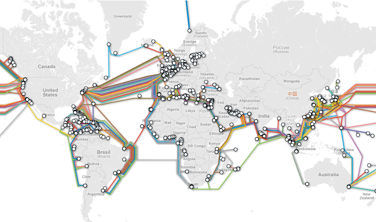
Every time a person or entity communicates over this network: information must be routed from the computer they start at, through a series of intermediate computers, then reaching a destination and starting the return trip. If Alexander was located in Bloomington, Indiana, USA and wanted to read content on the website associated with www.tu-darmstadt.de, then he would need to request the information before the website could respond with the information. Similar to how a written letter in the 1800s would pass from person to person, requests and responses between two computers must pass between computers and over wires.
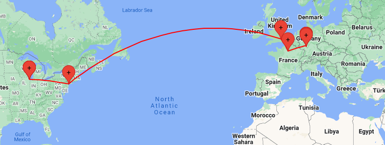
Addendum: traceroute
The
traceroutecommand (apt install traceroute) details which nodes and addresses sit between you and your destination.$ traceroute -I -q1 www.tu-darmstadt.de 1 hayesall (...) 2.571 ms ... 13 chi-b23-link.ip.twelve99.net (62.115.180.10) 18.726 ms 14 chi-bb2-link.ip.twelve99.net (62.115.126.158) 25.561 ms 15 nyk-bb2-link.ip.twelve99.net (62.115.132.134) 35.281 ms 16 ldn-bb1-link.ip.twelve99.net (62.115.113.21) 110.172 ms 17 prs-bb1-link.ip.twelve99.net (62.115.135.25) 119.136 ms 18 ffm-bb1-link.ip.twelve99.net (62.115.123.12) 120.602 ms ... 29 cms-sip02.hrz.tu-darmstadt.de (130.83.47.181) 130.942 ms
The Internet and the World Wide Web
What is the Internet then? The Internet is a series of connected computer networks with rules governing how computers on the network interact with one other.
The Internet is therefore an innovation in human communication. The physical and human infrastructure involved in that communication is no longer paper, hands, and ink: but system administrators, packets, and bits. This also means that when you overhear people complaining about “the Internet”—you can say to them: “Umm, technically, complaining about the Internet is like complaining about the postal service. You probably mean the world wide web.”
What is the world wide web then? It’s the interface, or the software running on servers connected to the Internet. The world wide web is what allows people to share information through links and through their interactions with web pages.
What we now call the world wide web (or www, but now often just called the web) was started by Tim Berners-Lee in 1989 at the European Organization for Nuclear Research (CERN). He originally referred to the project as the “Mesh”, and the “World Wide Web” terminology came about while actually writing the code.1 The reasons for creating the web were similar to the issues we used when motivating git: managing documents, sharing code, and preventing the loss of information. CERN followed a hierarchical tree structure (like we’ve seen on several different occasions): with engineers at the bottom, managers in the middle, and managers-of-managers at the top:
graph TB
C --- A;
C --- B;
A --- D;
A --- E;
Trees are excellent for organizing information—but hierarchies are a terrible way to organize people. Communication among people is network-structured. Have you previously worked somewhere? Did you have a boss? Was your boss the only person you ever communicated with?
The web, or “[t]he actual observed working structure” how people really communicate1 was Tim Berners-Lee’s answer to this problem, and it consisted of three key ideas:
- Hypertext (HTML). A means of representing content in an interconnected world. Documents written in a hypertext markup language could express arbitrary information, and would be discrete, referenceable nodes.
- Hyperlinks. A means of referencing or linking to other documents. Rather than following a tree structure: a link could reference anything, and a person following links could get to any document by following a chain of links back to the source.
- Hypertext Transfer Protocol (HTTP). A means of expressing actions over a network, such as getting a resource, posting a resource, or deleting something.
Perhaps more interesting is what the proposal left out. Hypertext is a means of representing information, not interpreting it, evaluating its relevance, or evaluating its truthfulness. Hyperlinks involve the name of a resource, but nothing about what to do when information changes. The protocol said nothing about security: the original assumption was that participants all knew and trusted each other (and secure HTTP—HTTPS—came many years later). We have hindsight—so more on those later.
Nevertheless, the most important thing was the generality of the three tools, and that good abstractions could be built on top of them. A person can be an observer to these three concepts. One does not even need to know what HTML, hyperlinks, or HTTP are. One can simply grasp the concept that they are looking at a document and following links—all while the protocol and servers work in the background to make it all possible:
graph LR
A --- B;
B --- C;
C --- A;
C --- D;
D --- E;
E --- C;
A --- E;
The very first web pages were written only in HTML and looked basic and were explored through command-line interfaces (CLI), but the concept of the web—connecting information with links—is still true today. The aforementioned abstractions turned into graphical user interfaces (GUI) browsers to help users navigate content.
The generality of pages, links, and protocols eventually meant the tools could be applied outside the niche interests of CERN, militaries, and governments—but would form an information infrastructure which could underlie everything else in the world.
Consider enrolling for classes in a world where the web does or does not exist:
- Before the web: enroll for class
- You can walk to Indiana University's registrar office, stand in line, talk to someone, request a paper bulletin, fill out a form with the class you want to take, drop off that form, and wait a week for the letter informing you that class is full.
- After the web: enroll for class
- You get Indiana University classes from the registrar's website. That website is connected to a database with real-time information about availability. You post a form telling the website which class you want.
Or consider traveling somewhere in a world with and without the web:
- Before the web: book a flight
- Flight information is scheduled and coordinated by airlines. You call an airline, or you solicit the services of a travel agent. The person you're talking with on the phone has a computer in front of them. That computer has a command-line application that helps them resolve your problem. You get a paper ticket mailed to you. If you lose the paper, you won't be allowed on the flight.
- After the web: book a flight
- You find a website that tracks flights from multiple airlines, and collates them according to price. You book a flight through an airlines website based on the time and price that works best for you. The ticket is a QR code stored in your phone.
The point, of course, is that many human problems are information problems. You want to do \(X\), but that first requires knowing about \(Y\), and informing another person or entity about your desire to do \(X\). Human hands, mouths, and minds can eventually move information information from one place to another: but an information system could instead be used to organize, access, and produce new information. Because an information system can fulfill these needs: many of the things that previously took hours, days, (or years) can instead be done in an instant.
Daily adult life, at least in a country like the United States, requires one to interact with interfaces to such information systems. Typically that interface comes via a website. Websites—the primary vehicle through which one accesses information on the web using the infrastructure of the internet—are therefore where we will concentrate for the rest of this book.
As Erika says: “Web interfaces are now the interfaces for our lives.” We’ve replaced checkbooks, paper forms, phone books, wall calendars, books, pens, paper, etc.. many of the physical items needed to run our households and manage our lives with web interfaces.
Programming concepts will not leave us: notice from our former examples that we had to look up information or sort results. The final website a user sees is like an iceberg: one will only see the 10% above the water. Our goal from this point forward is to see the whole iceberg: and build an information system.
Applications, or “apps”
But first, a brief diversion.
There were applications (now often shortened to apps) long before the web, and data storage predates computers by several millenia. That rock-paper-scissors implementation that we eventually called a “software package” evolved according to the same environmental pressures that made computers fundamental to daily life.
We started with a simple architecture: we asked for some user input, that input was translated into some internal “game logic”, and the product of the computer executing that logic was some output shown to the user.
graph LR
A[User Input] --> B[Game Logic];
B --> C[Show Output];
But we were unsatisfied with this mostly-stateless program. We wanted the program to also write, or store, its data to some location for later use.
graph LR
A[User Input] --> B[Game Logic];
B --> C[Show Output];
B -->|Write| D[File];
Finally we looped this data storage step back on itself. Not only could the application be affected by the user input: but problems like “showing a scoreboard” had to be based on external resources stored in files: meaning that program logic was now dictated by the present user input, but also the history of all past user inputs.
graph LR
A[User Input] --> B[Game Logic];
B --> C[Show Output];
B -->|Write| D[File];
D -->|Read| B;
This shows us that an application has three key components: an interface for input/output control, which drives the behavior of a back end implementing the logical core of the application, and a data store where application state is loaded from and saved to.
In rock-paper-scissors, we did not have a particularly clear demarcation between these three components. We implemented the application with a command-line interface where the input was a string, the internal states were predominantly managed with functions consuming and returning strings, and the output was (surprise!) a string printed to the console or saved to a file.
This approach to application design and information systems started around the 1890s with (what became) IBM tabulating the United States census. But like many human endeavors—the generality of the approach wasn’t recognized until many years later. And as we saw with Tim Berners-Lee’s pain points that led to him inventing the web: simple file input-output devices were not particularly helpful when it came to the challenges of networked human communication.
If only there were some way to link these two ideas: an “application” with a “decentralized networked interface”?
Not just a website, but a web application
Websites evolved. (And they continue to evolve: this story is not over, the web is younger than your instructors). (Oh great. Thanks for the reminder Alex. At least Erika knows what these emojis that stand for “old” mean ☎️ 💾 💽 📠 📼?)
Websites evolved from being simple HTML documents into the complex designs whose behaviors could mirror the needs of the information they were tasked with representing.
The sort of websites we previously covered still exist, but we now call them static sites. Here: static has two meanings. Its first meaning comes out of computer science jargon, where static refers to the case where an object has a fixed, unchanging size, and needs no context-specific information to reason about.2 If an HTML document is stored on a server as a static file, that file has a fixed size that can be measured in bytes. Computers are phenomenal when data are fixed and known: meaning that a website built from static files is scalable,3 and a static file server can handle tens-of-thousands (\(10e4\)) of concurrent users.
Static sites remain popular for content that changes relatively infrequently: such as personal websites, portfolios, blogs, or this book. The second meaning of static is to contrast the word dynamic. An object that is dynamic is either moving, or it is changing, or it is in some way responding to the world it inhabits. The time component in a dynamic equation. A dynamic site is therefore a site which is always in flux. Users can get information, but users can also change how the site behaves over the course of their interactions with it (like, post, subscribe, add, checkout, login).
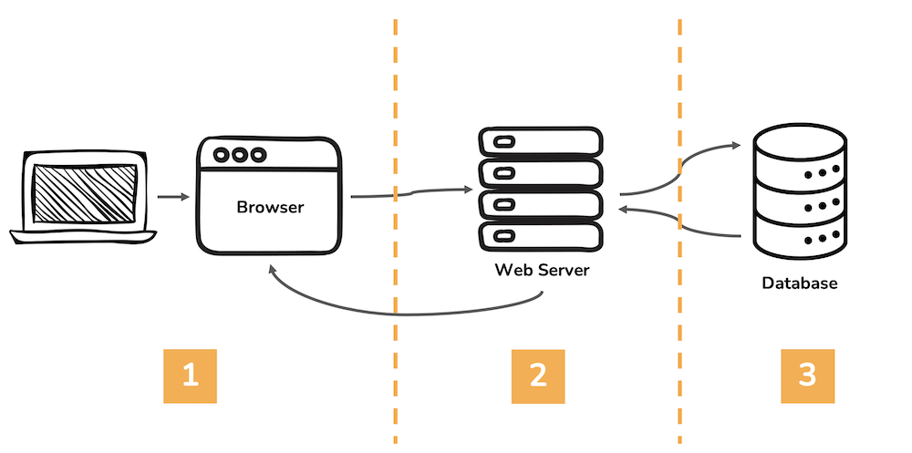
The three components that we said made up the web—HTML, hyperlinks, and HTTP—have little to say on how dynamic sites are built. But the basis for dynamic sites is buried within HTTP methods (or the HTTP verbs): GET or POST.
Web applications are made of three layers:
- An interface (frontend) - made of HTML, CSS and JS
- A framework (the control) - a programming language and an application framework, like Python/Flask - another popular combo you’ve probably heard of is JavaScript/React
- A database (backend) - we’ll be using MariaDB and SQL
In this unit, starting today, we’ll start with the interface and work our way through how to use the Flask framework. In the final unit, we will add in the backend.
The Request / Response Cycle
Because our interface is web-based, let’s first look at what happens after we type a URL into a browser and hit return:
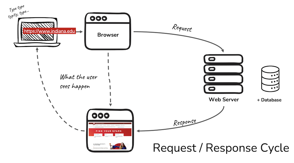
The user isn’t usually paying attention to what the browser is up to. A user’s main goal is to click a link or type in a URL and immediately access a web page with the desired information. A user MIGHT be vaguely aware that there is a web server (somewhere) (doing something) that the browser is connecting to.
What we as web application developers need to know is that when we click on a link, the browser initiates a two-step Request / Response Cycle in order to show you the linked page.
Using Your Browser as a Web Developer
- Watch the video to learn how to access the code behind the content in a web browser like a developer does. We’ll also take a look at how to see the request response cycle in action.
Step One: DNS
First, the browser uses the Internet to REQUEST the address for the URL submitted from a Domain Name Server (DNS). The URL is made up of friendly words, making it easier to remember and be understand by humans.
The DNS RESPONDS with an IP address (four sets of numbers separated by dots like this 129.79.7.128) based on the URL, telling the browser where to look on the Internet. Think of it as looking up a friend’s phone number in the Contacts on your phone. We maybe don’t remember the phone number, but we hopefully remember our friend’s name.
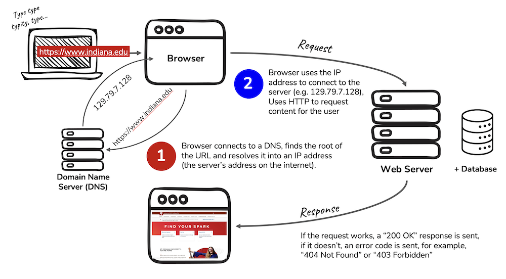
Step Two: Server
Second, the browser goes back out onto the Internet, now with an address in mind, to REQUEST data from a server (networked computer).
Once a connection has been made, the web server will RESPOND by sending the requested information in little packets of data until all of the data has been sent. As each resource for the web page come into the browser, a status code of 200 OK indicates the data was received.
Other possible status codes you might recognize are 404 Not Found and 403 Forbidden.
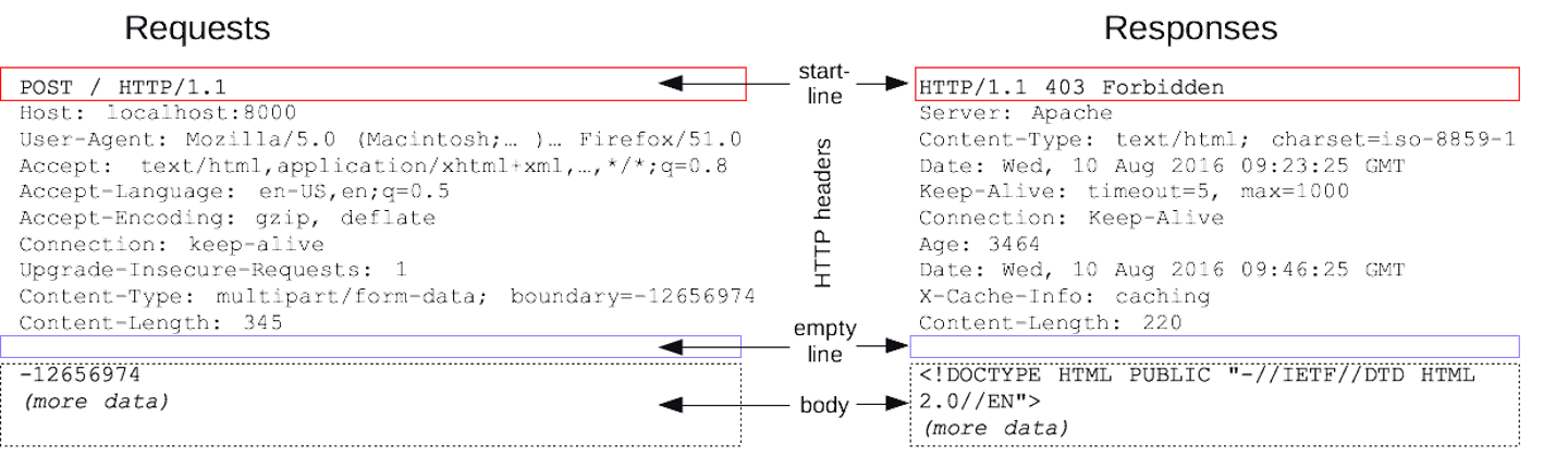
Assuming all goes well, the browser now takes any HTML, CSS, JS, images, etc.. sent from the web server and displays that content as a web page. And all of that happens in milliseconds.
The Request / Response cycle is fundamental to how browsers and the Internet (and later on, databases) interact. To see this interaction happening in the browser:
-
Open up the developer tools / web inspector in your browser. (how to do this)
-
Click the Network tab, then refresh the page to see a list of all of the requests and responses between the browser to the server. You’ll see columns of information showing the status code (most should say 200 OK), method used to send the data (GET is most common), and the domain (assets.iu.edu, or google, for example)
-
Scroll down in the list of requests/responses and click on one of the rows. You should information about the Header, Request and Response sent between the browser and web server.
Client-side versus Server-side
Let’s think about the second step - where the browser connects to the web server. There is a division here between technologies that work on the client-side and those on the server-side.
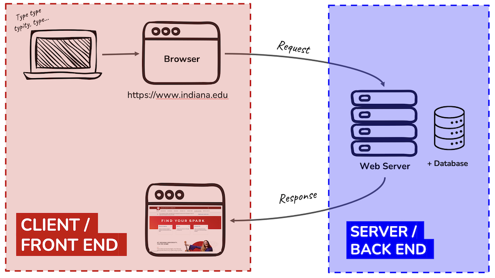
For each of the following, is this technology considered frontend (client-side) or backend (server-side)?
Make a guess before you reveal the answers.
- Python
- HTML
- CSS
- JavaScript
- SQL
- PHP
- Google Chrome Browser
- Apache Web Server
Technologies that work on the ‘frontend’
Frontend
HTML, CSS, JavaScript, and the Google Chrome Browser
Anything 'browser' like Firefox, Safari, etc.. is also here
Technologies that work on the ‘backend’
Backend
Python, SQL, PHP, and the Apache Web Server
Node.JS is a backend version of JavaScript, so if you put JS in this bucket, you are correct in that it can in a general sense do both
Anything 'server' (like Apache) or 'database' (SQL) related is here
Practice
Reminder from Networked Computers, Servers, and HTML: Websites about the structure for a simple website.
Set up
Continue to work out of your https://github.iu.edu/i211su2024/USERNAME-i211-starter today.
Note - your instructor is working just locally, no repo, the video was made before we had decided what repos to provide to you. So please work out of the same local repo you used for Rock Paper Scissors. You’ll be creating a folder for a simple static website today, and also a different folder for another static website tomorrow. You can run it locally (open the HTML files on your computer in a browser) to see what it looks like. No worries about pushing it to production or running on a web server. That’s what the end of this week will focus on when we start setting up Flask.
OK let’s go
Static websites have a simple tree-like data structure. Each item has only one parent, but that same item can have multiple children.
In HTML this structure is nested, with tags inside of tags. The outermost tag is <html>.
-
The
<head>contains information about a web page, along with resources such as CSS, fonts and sometimes JS. -
The
<body>is where all content we want to appear on screen lives, and is the more likely place for where JS lives. We want the HTML content to load and then the JS, so often you’ll find script tags at the very end of the BODY just before the close body tag.
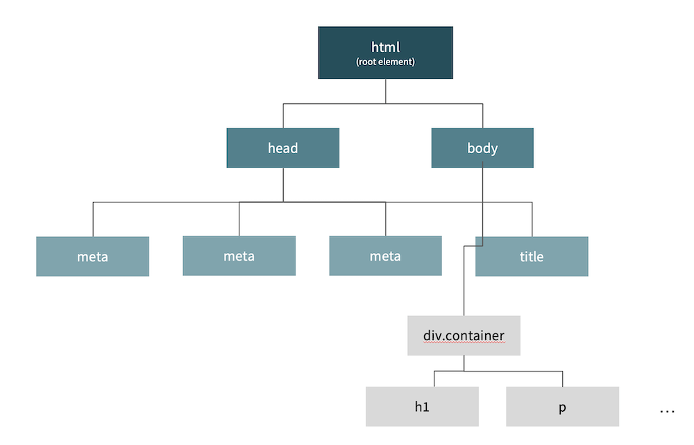
This image shows not only the required tags for an empty web page, but also where CSS, JS and other HTML should be placed.
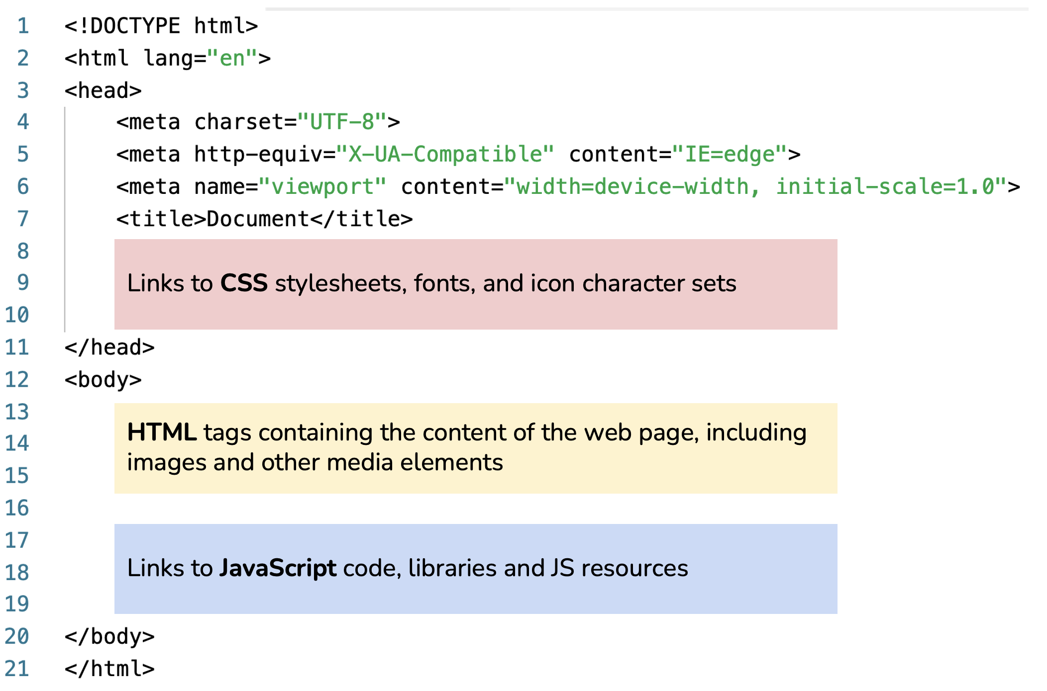
We’re going to build a static website (locally) with the goal of seeing how the HTML, CSS and JavaScript fit together to form a web page.
Note: Although we will write a bit of CSS today, nearly all of the CSS and JS in i211 will be taken care of by Bootstrap, a frontend framework providing styles and layout through class attributes for HTML tags.
Follow Along with the Instructor
Work through the practice with the instructor! This video goes into much less detail than what is written in the book, however, we also spend time on tips for VS Code, for example. You need both resources, it’s not a choose one or the other situation. 🤔
Building a Static Website
At the command line, change into the directory where your i211-starter repo is located. Set up a directory for a static site. Then open the repository in VS Code.
cd USERNAME-i211-starter
mkdir static-site
cd static-site
code .
Using the “New File” and “New Folder” buttons in VS Code’s Explorer to create the following file structure. Begin by creating a directory and naming it static-site. Note that images, css and js are all folders; index.html and level-up.html will be empty at first.
static-site
├── index.html
├── level-up.html
└── images/
├── html-css-js.png
└── flask-logo.webp
└── css/
└── js/
Place these two images into your images folder (right-click and save):

![]()
Set up a home page
Let’s start with index.html, the home page.
- Open the Bootstrap documentation
- Under ‘Quick Start’, copy the code under Step 2 Include Bootstrap’s CSS and JS and paste this into
index.html. Make sure you save. - In VS Code, go to Extensions (fifth icon down on the left), then search for and click the green “Install” button to install Live Server by Ritwick Dey. (You won’t need to restart, go back to Explorer when done) You should now see “Go Live” in the bottom right of your VS Code window.
- Click “Go Live” - this will open a local webserver and display your page in your default browser. The page should say “Hello, world!”.
Live Server giving you trouble? You can also just navigate to the HTML page you made and double click on it within your operating system. It will open in your default browser. To see changes, however, you’ll need to refresh the page.
What are we looking at here?
The HTML code can be broken down into these distinct parts:
<!doctype html>
<html lang="en">
<head>...</head>
<body>...</body>
</html>
doctypetells the browser that this is modern HTML.htmltag to hold the pieces of the web page.
<head>
<meta charset="utf-8">
<meta name="viewport" content="width=device-width, initial-scale=1">
<title>Bootstrap demo</title>
<link href="https://cdn.jsdelivr.net/npm/bootstrap@5.3.3/dist/css/bootstrap.min.css" rel="stylesheet"
integrity="sha384-QWTKZyjpPEjISv5WaRU9OFeRpok6YctnYmDr5pNlyT2bRjXh0JMhjY6hW+ALEwIH" crossorigin="anonymous">
</head>
The head tag contains information and resources that are needed for the page, but do not appear in the browser window.
- sets character encoding to a universal character set
- page will make use of mobile design techniques
- sets a title to appear in a tab in the browser’s window
- links to Bootstrap’s CSS for styling and laying out content
<body>
<h1>Hello, world!</h1>
<script src="https://cdn.jsdelivr.net/npm/bootstrap@5.3.3/dist/js/bootstrap.bundle.min.js"
integrity="sha384-YvpcrYf0tY3lHB60NNkmXc5s9fDVZLESaAA55NDzOxhy9GkcIdslK1eN7N6jIeHz"
crossorigin="anonymous"></script>
</body>
The body tag contains all content displaying on the web page, plus a spot for any JavaScript needed for page interactions.
h1tag is a top-level headline used as the main title for a web page- JS is included in a
scripttag, and is always at the bottom of thebodytag, right before the tag closes. This link pulls in Bootstrap’s JS resources.
Add structure, content and an image to the home page
Let’s add some structure.
The main requirement for structuring a page is that your content needs to be inside a container controlling the width and position of the content.
- Open Bootstrap’s documentation under Layout for adding a container
- Copy the code for a default container, and place these tags around the
h1
<div class="container">
<!-- place H1 here -->
</div>
Now add an image to the home page.
- Open Bootstrap’s documentation for how to add images
- Copy the code for a “responsive image” - this means the image will expand and contact in size to accommodate wider and narrower viewports
<img src="..." class="img-fluid" alt="...">
- Paste this HTML underneath the
h1tag (inside of the container) - Anytime you see
...in Bootstrap, it means “add your stuff here”:- For
src, type inimages/html-css-js.png- we need a relative link meaning the path is from where the index.html page is to where the image we want is located. - For
alt, add a short description or name for the image, for example, “logos for html css and js.” This attribute is required for accessibility.
- For
Make sure you check your progress in the browser.
Link to another page
Next let’s add a link to the page, either a standard link or one that looks like a button:
<!-- ADD a text-based link -->
<a href="#">Level Up!</a>
<!-- OR make it look like a button -->
<a class="btn btn-primary" href="#" role="button">Level Up!</a>
- To make the link work, replace the hashsign
#in the HREF with the path to the nearby HTML filelevel-up.html.
Time to add some style to the content.
Take a look at Bootstrap’s documentation as you add these so you can understand how to apply the code from their examples to our project.
- Add Spacing: Push the content away from the top of the page by adding the class
mt-5 - Center some text: Center the headline on the page with the class
text-center - Center an image: Center an image on the page with the classes
d-block mx-auto - To center the button, place it inside a DIV and use
text-center.
<div class="container mt-5">
<h1 class="text-center">Hello, world!</h1>
<img src="images/html-css-js.png" class="img-fluid d-block mx-auto" alt="logos for html css and js">
<div class="text-center">
<a class="btn btn-primary" href="level-up.html" role="button">Level Up!</a>
</div>
</div>
Make a second page
Finally, add a second page. A website isn’t much of a website if it doesn’t link pages together!
Repeat the process above on level-up.html to add an H1 and an image.
This time:
- H1 says “Level Up!”
- Image is set to
flask-logo.webp - Link directs to Flask’s documentation (https://flask.palletsprojects.com/en/3.0.x/)
Once again, make sure you check your progress in the browser.
Summary
We created a simple, static website using Bootstrap. Things to notice:
- The CSS and JS folders are empty!
Using Bootstrap means we don’t need to add our own CSS or JS unless we want to add custom styles or interactions.
- The HREF in a link is different for pages INSIDE and OUTSIDE of the site.
Linking to a page in my site means using a relative link - one that is based off where the HTML file lives in the file structure. Whereas an external link needs the whole kit and caboodle (the full URL including “https://”).
- The
level-up.htmlpage has a hyphen in the filename!
In HTML, the filenames often end up in the URL, thus names with multiple words are separated by DASHES. (In Python, we use underscores. This stylistic difference can be annoying to remember, but will ultimately help us tell the difference between code for the front-end and code for the programming or database portions of our web app.)
Footnotes
Berners-Lee, Timothy J. (1989). “Information Management: A Proposal (No. CERN-DD-89-001-OC).” Online. Accessed 2023-06-13. https://www.w3.org/History/1989/proposal.html
This is the static in public static void main.
Without diving into computational complexity theory: an algorithm is scalable when adding one additional computer provides one additional unit of work—without severe diminishing returns.
CSS, Styling, and Bootstrap
In programming, we said it would be annoying if we had to re-invent the wheel every single time we wanted to do something. Therefore: some bright people designed module systems and standard libraries to package up the sort of tools we find ourselves using over-and-over-and-over again.
Our current goal is to build the interface for a web application. We could approach this in way we did in our original HTML and CSS practice: write content in HTML, then style the content using cascading style sheets (CSS) until we’re satisfied. Alternatively: what if we were equally annoyed by hand-writing HTML and CSS in the same way that it would have been annoying to write a random number generator from scratch every time we wanted to pick a random number?
Enter: components (in a moment).
The field of web design is concerned with how one builds user interfaces for the web. A web designer (similar: front-end developer or front-end engineer)1 works from the foundations provided by HTML, CSS, and JavaScript—and their goal is to build user interfaces. A “good user experience” is that goal. But recall the foundational tools are good for content (HTML), styling (CSS), and interactivity (JavaScript). We might say these tools are low-level. Each are responsible for how things are actually accomplished—but seen several occasions where working at a higher level of abstraction can give one a huge productivity boost.
For example, HTML has generic tags for common elements like headers, buttons, and dividers:
<h1><button><div>
But what about this next thing? Is there an HTML tag for it? Can you name this thing?
This thing is called a modal, or sometimes a dialog box. Modals, accordions, cards, spinners, and tooltips are all things that do not exist in HTML.2 But one can create these by combining HTML and CSS. In other words, each of these things are components: re-usable bits of an interface that may require multiple HTML tags, some custom CSS, and JavaScript to realize the full suite of user interactions on the component.
One approach to user interface design and development works like this: first construct a set of components around a consistent style, then anyone can apply those techniques to any new interface. This is realized through a front-end framework (also called frond-end toolkit or front-end design framework). Variations exist between frameworks,3 but their common goal is is to bundle components and simplify interface development.
The front-end framework we will focus on is Bootstrap. Bootstrap was originally created at Twitter (a social media site popular in the 2010s) as a set of re-usable CSS classes to give Twitter a consistent look. The 2010s were a critical period following the release of the iPhone (2008), and Bootstrap popularized an approach to creating sites with a consistent look-and-feel whether the user was viewing the site from a small screen (mobile device), a medium-sized screen (laptop), or a large screen (desktop). Anyone who has interacted with the world wide web has seen the results of using Bootstrap—the framework is currently being used on 17.7% of all websites.4
High usage suggests two observations. (1) When a tool is popular: it’s solving a problem many people have. (2) Using Bootstrap means you will have a functional, but generic-looking site. We will spend this chapter on a few topics:
- CSS. Enough of an introduction to cascading style sheets that one can recognize how the language is formatted, how the rules work, and how they may be applied to styling user interfaces.
- Bootstrap. A front-end framework with easy-to-use CSS rules. It contains some JavaScript, but the JavaScript can mostly be treated as a behind-the-scenes implementation detail.
- Emmet. A toolkit of snippets and shortcuts to use when writing HTML and CSS. Emmet is included as a built-in plugin for Visual Studio Code. We will introduce some of these as they arise, and recommend trying out some listed in the Emmet cheat sheet: https://docs.emmet.io/cheat-sheet/.
Separating Content from Style
If a web page were a storybook; then the HTML is the content of that story, displayed in a clear hierarchy of: chapters, their titles, and their paragraphs. The CSS is all about the adjectives, adverbs, and descriptive language that make a story memorable. The content is important, but a presentation style is what the user recognizes in their first-person journey through a web page.
We previously saw HTML and CSS when we introduced networks and servers, and introduced HTML tags to represent common types of content:
| HTML Tags for Content | Purpose / Meaning |
|---|---|
<p> | paragraph / default text container |
<h1> | headlines in order of importance |
<ul> | bulleted list / unordered list |
<ol> | numbered list / ordered list |
<li> | list item |
<table> | define table |
<a href="...">...</a> | create a table: row / cell (column) / header |
<img src="..." alt="..."> | place an image |
We learned that there was a generic <div> or “division” to incorporate structure or design elements, but likely were left uncertain about where and how they were used. Furthermore, there were a large number of tags that the introduction implied were important for building web pages, but were not defined until now:
| Required HTML Tags | Purpose / Meaning |
|---|---|
<!DOCTYPE html> | identifies page as HTML |
<html lang="en"> | wraps around your entire web page |
<head> | contains the stuff you don’t see on the page, but need: typically metadata or other machine-readable information |
<meta charset="UTF-8"> | define the page’s encoding to inform the browser how to render specific types of text |
<title>...</title> | title for your website/webpage shown as the title of a browser tab |
<link rel="stylesheet" href="..."> | links your HTML to your CSS (stylesheet) |
<body> | contains the stuff you do see on the page |
The CSS handles the styling and layout of the HTML tags in a web page. Best practices typically recommend to add CSS to its own file (since multiple HTML documents will need to refer to it), and to link the common stylesheet in the <head> of a document. For example:
<link rel="stylesheet" href="css/styles.css">
CSS is designed as another markup language. Each object in the language is a CSS rule informing a web browser how an HTML element (or the page more generally) should appear. Each CSS rule is like the dictionaries we saw in Python: where we mapped a key to a value—the same thing is true here, except in CSS they are called properties and values. The parts of each object are the:
- Selector. A selector corresponds with a specific piece of HTML, usually at the level of tags. A selector is accompanied by braces (
{}, sometimes called curly braces) which demark which selector(s) which are being modified. - Properties. The properties, attributes, or behaviors being modified, usually generic concepts like something’s “color” or “size”.
- Values. The actual value that an attribute takes on. If the attribute is “color”, its value might be set to “orange”.
The combination of a property and a value is a declaration. Declarations use a colon : to separate the property from the value, and end with a semicolon ;. Quiz yourself with the following, what is h1, what is color, and what is center?
h1 {
color: orange;
text-align: center;
}
Answer: h1, color, center
h1is a selector: it corresponds with an HTML elementcoloris a property: it corresponds with the way that an element is showncenteris a value: it is a specific way to display the text
More often, CSS rules are given meaningful names called CSS class selectors. In this context, a class is the adjective that modifies how one interprets the HTML nouns. An HTML document containing an article may benefit from having specific types of paragraphs; a lead-in paragraph might need to be styled differently from a generic paragraph, and styled differently still from a concluding byline at the end. Once defined in CSS and loaded (<link>) in an HTML document, a class can be applied to an element using the class= attribute of an HTML tag:
<p class="lead-in"> ... </p>
<p> ... </p>
<p class="by-line"> ... </p>
Analogous to how we saw dot notation or attribute-based indexing in Python, CSS classes also use a period/dot character to define new classes. If we define lead-in and by-line classes on the <p> element:
p.lead-in {
font-style: italic;
}
p.by-line {
font-style: italic;
font-size: 18px;
}
… then attribute and value settings will only apply to paragraphs with those classes:
So what is the takeaway from this? We will not spend much time on CSS in this book. You should, however, be able to recognize CSS code when you see its basic syntax and application. As we mentioned: Bootstrap will handle basic styling and layout with a set of prewritten CSS classes. Therefore the takeaway is that Bootstrap abstracts away the need to write some of the CSS, allowing the interface developer time to focus on the final presentation. We will instead spend time learning how to apply Bootstrap classes from within HTML: and recommend returning to the low-level styling details as a topic for another time.
Bootstrap Classes and HTML
Adding Bootstrap to a site can be as simple as including CSS and JavaScript links via <link> and <script> tags, respectively. From Bootstrap - Get started :
<!doctype html>
<html lang="en">
<head>
<meta charset="utf-8">
<meta name="viewport" content="width=device-width, initial-scale=1">
<title>Bootstrap demo</title>
<link href="https://cdn.jsdelivr.net/npm/bootstrap@5.3.3/dist/css/bootstrap.min.css" rel="stylesheet" integrity="sha384-QWTKZyjpPEjISv5WaRU9OFeRpok6YctnYmDr5pNlyT2bRjXh0JMhjY6hW+ALEwIH" crossorigin="anonymous">
</head>
<body>
<h1>Hello, world!</h1>
<script src="https://cdn.jsdelivr.net/npm/bootstrap@5.3.3/dist/js/bootstrap.bundle.min.js" integrity="sha384-YvpcrYf0tY3lHB60NNkmXc5s9fDVZLESaAA55NDzOxhy9GkcIdslK1eN7N6jIeHz" crossorigin="anonymous"></script>
</body>
</html>
When Bootstrap is added to your site, its pre-written CSS applies automatically. Furthermore, specific CSS classes may be applied to your HTML elements in the form of class attributes. A class attribute applies a CSS class selector to an HTML tag, such as the <p class="lead-in"> that we showed earlier. Bootstrap classes are typically applied in four ways, which we’ll call the:
- Reset,
- Singleton class,
- Multi-class/Mixin, or
- Component
… approaches. This vocabulary comes up throughout web development. We’ll provide brief examples of each in Bootstrap. But for most day-to-day problems: one can usually pick up which one is correct in which situation by reading examples from documentation.
Bootstrap Reset
Bootstrap provides default styling: As a web designer, you can apply zero classes to an HTML element and Bootstrap will apply some default styling. If you aren’t using Bootstrap, every web browser also has a built in stylesheet, but it’s very basic. This approach is sometimes called a Reboot or CSS Reboot (e.g. Bootstrap Reboot ), because overwriting every web browser style effectively resets behavior to some other state, making appearance consistent across browsers.
Without a single class—Bootstrap changes everything from font, to its size, to the document’s background color:
Bootstrap - Singleton Classes
Singleton classes modify a specific HTML element to look a certain way. If you can express an idea like: “big heading”, “opening paragraph”, “unstyled-list”, etc., the concept is usually implemented by adding a class="..." to a desired HTML element.
Notice in the following how classes are set in the opening HTML tag and never in the closing tag? Notice how there is a space between the name of the tag p and the attribute class="lead", but no spaces within the attribute syntax?
<h2 class="display-5">The Bootstrap Reset</h2>
<p class="lead">
A reset, or browser reset, shadows the default CSS
used by browsers.
</p>
Applying classes like these change how particular elements are displayed by the browser. When building interfaces (or sites more generally), these extend the HTML vocabulary with variations on concepts:
Bootstrap - Multiple Classes and Mixins
One can apply multiple classes to an HTML element. Just put a space between the class names. This is sometimes called a mixin approach—because one creates a desired effect by “mixing together” multiple simple classes.
For example: Alexander felt claustraphobic looking at the previous examples—with the text crammed against the left and top of the screen. It would look nicer if there was some spacing at the top, and equally on the left and right sides. This could be fixed by wrapping everything in a <div> element with a medium margin at the top: mt-3, and a container to handle left and right spacing.
<div class="container mt-3">
<h2 class="display-5">The Bootstrap Reset</h2>
...
</div>
Much better:
Bootstrap - Components
Components are higher-level pieces of an interface which combine aspects of the three previous ideas. Components are also one of the biggest productivity advantages to using a framework like Bootstrap, particularly if one needs things like forms, modals, navigation, or other heavily user-driven elements.
For example, the Bootstrap Modal that we saw earlier is created by applying the modal singleton class, then the position-static and d-block mixins. Within a modal: there are additional steps to express the modal-content, modal-header, modal-title, and even more attributes (e.g. “data attributes”) to fine-tune their behavior.
Do you have to memorize all of these? No! But there is a lesson to be learned for everything we have seen so far: The documentation is your friend. Experts with years of experience working on Bootstrap probably know everything in the documentation, but when you’re starting out: leveraging that expert knowledge typically requires reading documentation. Enough that you can read an example such as this:
<div class="modal position-static d-block" tabindex="-1">
<div class="modal-dialog">
<div class="modal-content">
<div class="modal-header">
<h5 class="modal-title">Confirm?</h5>
<button type="button" class="btn-close" data-bs-dismiss="modal" aria-label="Close"></button>
</div>
<div class="modal-body">
<p>Make sure you save your changes first.</p>
</div>
<div class="modal-footer">
<button type="button" class="btn btn-secondary" data-bs-dismiss="modal">Close</button>
<button type="button" class="btn btn-primary">Save changes</button>
</div>
</div>
</div>
</div>
… and intuit how it translates into the user seeing this:
JavaScript and Interactive Components
Soon we will need to figure out what “interactive” means—but not yet. HTML and CSS are layout and styling languages. Interactivity—the means by which someone uses an interface to accomplish their goals—requires us to “wire up” the front end of an application to something that actually implements the logic.
The way one “wires up” components on the front end to a programming language typically goes through a few HTML attributes:
idnamedata-*
Briefly: Bootstrap might make use of the id attribute of a component to make them interactive. Flask will make use of the name attribute. Finally, data-* attributes configure Bootstrap plugins and hold behind-the-scenes data for specific components (for example, the modal example included a data-bs-dismiss attribute to annotate which buttons the user could click to dismiss the modal).
Such an element uses multiple attributes, similar to:
<div class="dropdown" id="action-items">...</div>
In context, notice how the following <form> element contains an <input> and <label>. Both refer to a userEmail identifier: defined in the input, then used by the label.
<form class="form-floating">
<input
type="email"
class="form-control"
id="userEmail"
name="userEmail"
placeholder="name@example.com">
<label for="userEmail">What's a good email for you?</label>
</form>
Some Concluding Remarks
To reiterate: it’s not important to memorize the classes and ids to use—Bootstrap’s documentation will tell you. Focus instead on what you want to show to a user, translate that into something in Bootstrap (Grid, Images, Tables, Select, Button), and how to adjust an example to fit a new use case.
In documentation, you will typically see:
...- dot-dot-dot is a placeholder for you to fill inExample- represents a name you’ll want to change<a href="#">- hashsign should be replaced with a relative path or a URL
Follow Along with the Instructor
Practice with the instructor and learn some more VS Code shortcuts. As always: the video is not an exact replacement for the written directions and vice versa.
Practice
Today we will create a “cheat sheet” web page linking to parts of the Bootstrap documentation, practice centering, and practice the Bootstrap grid:
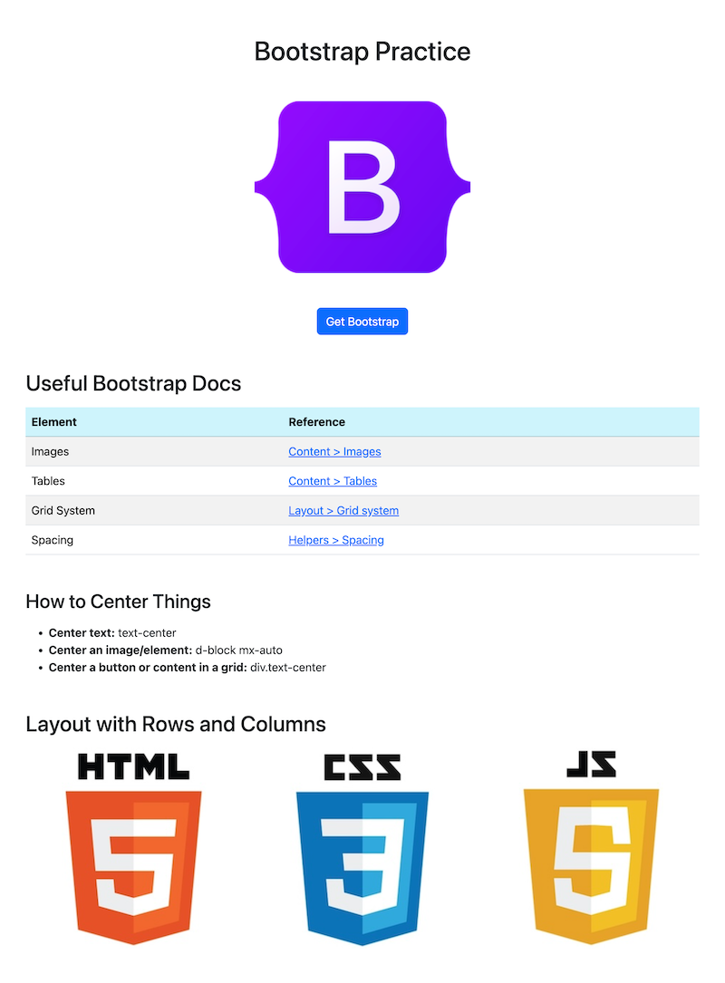
01 Open the Bootstrap Documentation
Open the Bootstrap documentation. Take a look around. As concepts come up during practice, find a relevant section of the documentation: either with the “Search” functionality, or using the table of contents along the left side of the screen.
02 Set up
Continue to work out of your https://github.iu.edu/i211su2024/USERNAME-i211-starter today.
At the command line, change into the directory where your i211-starter repo is located. Set up a directory for a static site. Then open the repository in VS Code.
cd USERNAME-i211-starter
mkdir bootstrap-practice
cd bootstrap-practice
code .
Note - reminder that your instructor is working just locally, with no repo, the video was made before we had decided what repos to provide to you. Continue to work out of the same local repo you used for Rock Paper Scissors. You’ll be creating a folder for another static website. If Live Server doesn’t work for you, run it locally (open the HTML files on your computer in a browser) to see what it looks like. No worries about pushing it to production or running on a web server.
We’ll work with just one HTML page today and a simplified structure so we can focus on practicing with Bootstrap.
In bootstrap-practice, create the following file structure:
bootstrap-practice
├── practice.html
└── images/
03 Download a logo to use in the site
Right-click to download the image.

Drag the image (maybe from your computer’s “Downloads” folder) into the images/ folder we just created. Your site structure should now look like this:
bootstrap-practice
├── practice.html
└── images/
└── bootstrap.png
04 HTML Boilerplate and Bootstrap
Add this HTML to practice.html:
<!doctype html>
<html lang="en">
<head>
<meta charset="utf-8">
<meta name="viewport" content="width=device-width, initial-scale=1">
<title>Bootstrap Practice</title>
<link href="https://cdn.jsdelivr.net/npm/bootstrap@5.3.3/dist/css/bootstrap.min.css" rel="stylesheet"
integrity="sha384-QWTKZyjpPEjISv5WaRU9OFeRpok6YctnYmDr5pNlyT2bRjXh0JMhjY6hW+ALEwIH" crossorigin="anonymous">
</head>
<body>
<!-- Add content here -->
<script src="https://cdn.jsdelivr.net/npm/bootstrap@5.3.3/dist/js/bootstrap.bundle.min.js"
integrity="sha384-YvpcrYf0tY3lHB60NNkmXc5s9fDVZLESaAA55NDzOxhy9GkcIdslK1eN7N6jIeHz"
crossorigin="anonymous"></script>
</body>
</html>
05 Add content to the body
Add this code to the body of practice.html:
<div class="container mt-5">
<h1 class="text-center">Bootstrap Practice</h1>
<img src="images/bootstrap.png" class="img-fluid d-block mx-auto my-5" alt="bootstrap logo">
<div class="text-center">
<a class="btn btn-primary" href="https://getbootstrap.com/" role="button">Get Bootstrap</a>
</div>
</div>
Pay attention to:
- In Bootstrap, content goes inside a “container” class
img: a relative pathname is used for the image’s source, meaning the path based on where the HTML page lives in relation to the image we want to appear- The content is being centered using three different techniques
- Notice that spacing is handled by classes beginning with an “m” (more on that soon)
To view the page, click “Go Live” in the bottom right corner of VS Code.
06 Add a table of documentation links
Hint: In the Bootstrap Documentation go to Content > Tables
- Add an
h2called “Bootstrap Docs” - Add a
tablewith atheadand atbodytag similar to the one in the first example in the documentation - In the
thead, place a row with two table heading (TH) columns called “Element” and “Reference” - In the
tbody, place four rows and add the following content:
Images
Content > Images
https://getbootstrap.com/docs/5.3/content/images/
Tables
Content > Tables
https://getbootstrap.com/docs/5.3/getting-started/introduction/
Grid System
Layout > Grid system
https://getbootstrap.com/docs/5.3/layout/grid/
Spacing
Helpers > Spacing
https://getbootstrap.com/docs/5.3/utilities/spacing/
07 Add a list of tips
Hint: In the Bootstrap Documentation, look for Layout > Grid
- Add an
h3with the title “How to Center Things” - Create an unordered list with the following content:
Center text: text-center
Center an image/element: d-block mx-auto
Center a button or content in a grid: div.text-center
08 Create a grid of images
Add an h2 with the title “Layout with Rows and Columns”
Right-click to download the following three images, put them in our site’s images/ directory.


Add the following code and use the documentation to figure out what these classes mean:
<div class="row g-3 text-center">
<div class="col-12 col-md-4">
<img src="images/html.jpg" alt="html">
</div>
<div class="col-12 col-md-4">
<img src="images/css.jpg" alt="css">
</div>
<div class="col-12 col-md-4">
<img src="images/js.jpg" alt="js">
</div>
</div>
Solution: what do the classes mean?
In the final listing with rows and columns:
- the most basic row and column setup includes the
rowclass wrapped around one or morecolclassesg-3provides a medium sized gap between the elements (values are from 1-5)text-centercenters the table on the screenBootstrap provides columns made of up to 12 pieces. This allows for you to set a column to be full width (12), half width (6), a third (4) or a quarter (3) of the row.
col-12means that in a mobile view, each column will stretch to fill the entire rowcol-md-4means when the viewport is a medium width, each column will fill a third of a row
09 Adjust the spacing
In the Bootstrap Documentation, go to: Utilities > Spacing
- On all
h2orh3headlines, add a level 5 amount of margin on the top, and a level 3 amount of margin on the bottom. - On the
row(the last element in our content, has a class “row” applied), add a level 5 amount of margin to the bottom.
Hints: Bootstrap Spacing Formula
Spacing in Bootstrap has a formula. To understand this formula, we need to be aware of the two areas where space can be added.
- margin - the space around the element
- padding - the space between the content and edge of the element
(The border can be set to be visible, but is not set by default)
We also need to understand that all elements are boxes!
Whether we see the edges of that box or not, all tags are creating a box. The sides of an element can be set all together, or as a pair like top-bottom or left-right , or individually as top, right, bottom, and left.
10 Review and final fixes
Review your site so far and make any additional changes to tidy up its presentation.
When complete: commit and sync your changes with your GitHub repository.
(Bonus) Aesthetic preferences
Bootstrap provides many variations on the vanilla elements. Different preferences have associated classes mentioned in the documentation.
- Can you make the table striped?
- Can you give a hover effect to each row of the table?
- Can you change the background color for the
theadrow? - Can you make the first part of each list item either bold (
strongtag) or italic (emtag, for emphasis)?
Further Reading
- MDN Web Docs: Getting Started with HTML
- MDN Web Docs: HTML tag reference
- MDN Web Docs: Class selectors
- Bootstrap - Getting Started: JavaScript: Data Attributes
- MDN Web Docs: id
- MDN Web Docs: data
- MDN Web Docs: Using data attributes
Footnotes
There are distinctions between the roles of web designer, front-end developer, and front-end engineer: but in an introduction we will mostly treat these as aspects of the same end goal. Many roles in computing blur into each other, as roles are often problem-specific or team-specific. A front-end developer on a team with three people might be the only person who knows about user interfaces, implying many responsibilities. When these roles do have strong demarcations between them (read: on large teams) a designer works directly with end users to come up with an interface, a developer implements it, and the engineer connects the two (even if requires inventing new approaches or frameworks that didn’t exist previously).
In the next few years we may think differently about this modal example. As we mentioned: the HTML standard is evolving, and as of 2022 the <dialog> element was implemented by all major web browsers. Nevertheless, older devices still exist, and may not support the new features. Because of this: components built from better-supported tags remain common. See also: https://developer.mozilla.org/en-US/docs/Web/HTML/Element/dialog
Writing that “variations exist between front-end frameworks” is an understatement. It’s like saying that “variations exist between programming languages”—vacuously true to the point of sounding ridiculous. Bootstrap is a batteries included framework: supporting many pre-built components, and general grid, font, and sizing approaches. In a course that goes beyond this cursory introduction: front-end frameworks like React, Vue, Svelte, Solid—there are too many to name—are designed to build user interfaces, but also to handle some of the trickier parts around creating new components. In other words: they are designed to handle the state management problem we’ve seen several times. We avoid state management on the front end, as it is a topic for a class that goes deeper into JavaScript.
“Usage statistics and market share of Bootstrap for websites”, W3Techs. Accessed: 2024-07-02, Online: https://w3techs.com/technologies/details/cs-bootstrap
Server Routing in Flask
Today we are going to work on building a web application in class that is very similar to what we will ask you to do for your course project. We’ll continue to work on this site throughout the rest of the semeester.
The in-class web app is a recipe website called “🍳 Make This Now!” A repository of the code for this site will be provided, so don’t worry about the code – worry about whether you understand what the code does, and how to apply the techniques we are learning to your own project.
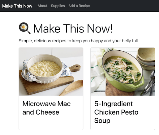
Do not skip this practice.
This web app we will build together IS YOUR PRACTICE. That time and effort will keep you from hours upon hours of wasted time and frustration when you then work on your course project. The risk is low, and the reward is high.

We have to do what??
We now have a passing familiarity with the essential technologies needed to build a web application with the Flask framework:
- Unix / Command Line and understanding a parent-child tree-like data structure
- HTML + Bootstrap (which includes CSS & JS) for the interface
- Server access (Silo) - so we have somewhere to place our application
- Git & Github - for source code management and keeping track of versions
- VS Code - a code editor that can handle multiple file types
- Python - our programming language - including how to test code, work with modules, handle structured data, and read / write to files
- Flask - our application framework - that we set up with
pipandvenv
(By the end of the semester, we will have added two more items to this list - SQL and databases - to handle the backend of our web application.)
Wheh. Creating a web application is a lot of work, and involves a lot of techniques and technologies.
So why bother?
Why not just make a static website using HTML, CSS and JS?
Why Creating a Web App is Useful
People build large, scalable websites (web apps) when they want to:
- make use of a database - more on that in Unit 3
- reuse parts of the code - for example when a navigation bar is repeated on multiple pages
- have more control over the URL - and exactly what is displayed on each page depending on the circumstances
These are all reasons to choose a web application framework. In this chapter, we are going to talk about item three,“we want more control over what is displayed when”, which is called Routing.
Note: you absolutely can make a simple website with just HTML, CSS, and JS. In fact, many projects are not large enough or complex enough to justify the setup time needed, but sometimes there might be a framework already in place, or the pressure to use the new shiny thing wins out. (Cause it’s shiny ✨)
Routing
Routing allows us to control what happens in our application when the the user clicks a link.
In a simple website, when a user clicks on a link and the browser loads the page. THERE IS NO MIDDLE STEP.
In a web application, that step in-between the user’s click and the browser loading a page is THE MOST IMPORTANT STEP.
- The user SEES 👁️ what they want to do on the site and clicks a link.
- Think of the
app.pyfile as the BRAIN 🧠. Decisions are made related to data and content. - Then the browser has a HAND 👋 in making it all happen.
What happens in a route?
This routing process consists of directing these three steps, starting with the user interaction:
- User clicks on a link
- This directs to a function in our web application (
app.py) - The function displays (renders) the desired HTML page
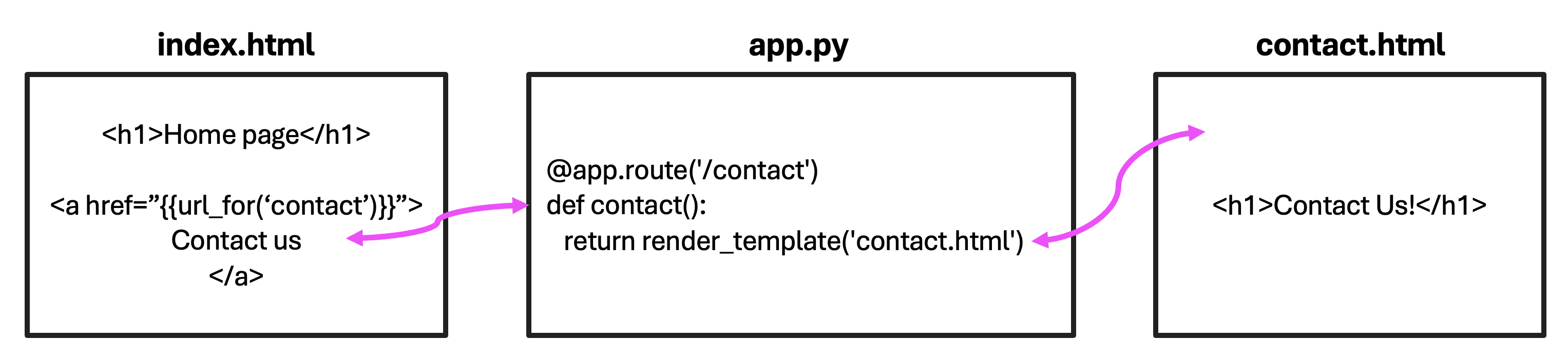
The link the user clicked on, in this case, resolves to a URL that looks like http://127.0.0.1:5000/ locally, or perhaps with its own URL, like https://www.make-this-now.com/, if it’s hosted on a web server.
In our app.py, the function contact() is called, which in turn returns a call to a function (render_template()), which display the web page contact.html in the browser.
We code this process in app.py like so:
@app.route('/contact')
def contact():
return render_template('contact.html')
Formatting a route
You may have noticed the word ‘contact’ is used three times; once for the route, once for the function and once for the HTML page displayed. We have three different parts and they all have the same name?!
It’s true, and we could write the route like this to avoid that:
@app.route('/contact')
def show_contact():
return render_template('contact-info.html')
The names DO NOT have to exactly match. There is no requirement that they do. However, it can often make sense to do so, and you’ll find this is a common practice, because we will have a lot of names to keep track of and it is easier to tell which pieces need to be connected if they all have the same name.
Now you know 💫 and can choose the convention that makes the most sense to you.
Where do routes live in my application?
Routes live in the flaskapp directory of your starter project in a file called app.py.
app.py
# Copyright © 2023-2024, Indiana University
# BSD 3-Clause License
from flask import Flask, render_template
app = Flask(__name__)
@app.route("/")
def index():
return render_template("index.html")
-
At the top of
app.pyis a line importing Flask, followed by a library we will need -
The next line creates a Flask data object that will help us control our application.
-
The first use for this
appobject is to make a route for the home page. (Notes: The@indicates this is Python decorator.\means the root of the file structure. And remember the home page for any website is usuallyindex.html.)
These last three lines of this code are saying when the user clicks on the URL for our website (e.g. “https://www.make-this-now.com”), we want our application to DO SOMETHING. Action implies verb, which in programming means a function. What do we want the function to do? We want it to display the home page index.html.
Want another page in your web app? Make another route. Just add it underneath the previous route.
@app.route('/about')
def about():
return render_template('about.html')
We can add as many routes to our application as we would like to.
Routes are activated by the user
Not all routes will run all the time. For the route code in the app.py to run, the USER CLICKED A LINK. 😮 (Or maybe directly typed in a URL, but usually the former.)
Think of the code in app.py a set of directions for what happens when a user interacts with a page in our website. This means when we go to test each route, we have to interact with the site’s interface to kick off each coded interaction.
Routes allow us to control what the URL looks like
Notice that the ROUTE name is a little different than the HTML page (or URL) displayed at the end of this interaction. One is “about” and the other is “about.html”.
- route - https://www.make-this-now.com/about or http://127.0.0.1:5000/about locally
- function - about()
- HTML template - about.html
This means in our Flask web application the URL DOES NOT look like
https://www.make-this-now.com/about.htmlbut ratherhttps://www.make-this-now.com/aboutbecause of how the ROUTE is structured. Locally, that’shttp://127.0.0.1:5000/aboutand NOThttp://127.0.0.1:5000/about.html.
url_for()
Adding a link to a simple website looks like this:
<a href="contact.html">Contact Us</a>
Adding a link to a Flask web application looks like this:
<a href="{{url_for('contact')}}">Contact Us</a>
All links in your web application will look like the second one!
How to add a link in a web app
Here is the approach your instructors take when adding a link in a web application.
First add the link in your HTML
- STEP ONE: Add double curly brackets between the quotemarks for the href attribute
<a href="{{}}">Contact Us</a>
- STEP TWO: Add the function url_for()
<a href="{{url_for()}}">Contact Us</a>
- STEP THREE: Tell the
url_for()function which FUNCTION we want to call in app.py
<a href="{{url_for('contact')}}">Contact Us</a>
Now we are good to go. When the user clicks this link in our web app, the function indicated in the url_for() will be called in app.py.
That’s right. The 'contact' inside of the url_for() function is THE NAME OF A FUNCTION. It does NOT represent the page you want the user to go to. We first have to go to app.py and connect to a function.
Next write the route
Now go to app.py and write the route:
@app.route('/contact')
def contact():
return render_template('contact.html')
The user may then notice that the URL at the top of the browser will change to say, for this example, “https://www.make-this-work.com/contact”.
Finish up by testing the route
And finally, the HTML page contact.html is displayed in the browser for the user to see.
Adding images and other static content
To add code and resouces used to make simple ‘static’ websites, we need to tell the web application where to look for such things as images, CSS, JS, etc… Because static resources are not processed dynamically the way our HTML will be (more on that in the next chapter), we can store them together in a folder called ‘static’.
flaskapp
└── static
├── css/
├── images/
└── logo.png
├── js/
└── favicon.ico
└── templates
└── tests
├── __init__.py
├── __main__.py
└── app.py
This is the structure for your flaskapp directory. We are going to need a way for the code controlling our application in app.py to access content in static. WE CANNOT (and should not) USE DIRECT PATHNAMES. Instead we want to allow the web application to do the work or resolving that pathname for us.
Flask provides us with a special function called ‘static’ that resolves to our static content folder without us having to write a special path. It does however need to then know the pathname for the resource WITHIN the ‘static’ folder.
For example:
<img src="{{url_for('static', filename='images/logo.png')}}" alt="logo">
Usually your static content will be sorted into folders by type of resource, so make sure you put a relative pathname into filename based off of ‘static’ as the root. (So images/logo.png is correct, and ‘logo.png’ or ‘static/images/logo.png’ are not in this example.)
This technique is how you will add CSS, JS, images and icons to your project.
Data In
What if we want to pass along some information from the web page where the user clicked to the web page where the user wants to go?
We can add a variable set to a value that shows up as part of the route, and can be accessed as a parameter in the function.
Sending data from a web page:
<a href="{{url_for('show_product', id=7)}}">Gizmo You Must Buy</a>
Notice the variable/value pair id=7. This data is sent along to the route when the link is clicked. You can add multiple variables (and values) here, just separate with a comma.
URL in the browser will change to:
http://www.some-website.com/product/7
When we get to the route in app.py we need to modify the code to grab this variable:
@app.route('/product/<id>')
def show_product(id="None"):
return render_template('product.html')
Notice the < > in the route? That’s how we indicate that part of the pathname is variable. What the route looks like in the browser depends on how it was sent from the link. In our example, id is set to 7. The pointy brackets do not appear when the route is presented as a URL.
To use the data in our function, we set it as a parameter. It becomes a local variable we can use as needed.
The variable name in the route MUST MATCH the name of the parameter!
In general, it’s also considered best practice to set the parameter to have a default value in case something goes wrong with the data coming from where the user clicked. We chose to make the value None in this example, and encourage you to do so in general, but you technically could set that default value to 0 or giraffe, or whatever you need.
Quiz Yourself: Given each route, what is the value of product_id in @app.route(’/product/<product_id>’)?
As in what would be set to the parameter product_id in show_product()? What would print?
@app.route('/product/<product_id>')
def show_product(product_id="None"):
print(product_id)
return render_template('product.html')
http://127.0.0.1:5000/product/IU-keychain
IU-keychain
http://127.0.0.1:5000/product/23
23
http://127.0.0.1:5000/product/
None
Since no value was set, the default is None
http://127.0.0.1:5000/product
None
Since no value was set, the default is None
http://127.0.0.1:5000/product/X329LV7?name="IU_coffee_mug"
X329LV7
The value is still in the same place. The 'query string' starting with the `?` is another way to pass data in a URL, but will be ignored in this situation.
Data Out
What if we want to pass this id number, or other data along to the page displayed in the browser when the function completes?
Sending data from the app to a webpage
@app.route('/product/<id>')
def show_product(id="None"):
username = 'Erika'
return render_template('product.html', username=username, id=id)
In this example, we are passing two pieces of data along to the page product.html – an id and a username.
- The structure for passing along data is variable-name-for-use-on-html-page is assigned to variable-coming-from-data-found-in-app.
- We can pass along as many pieces of data as we want at the end of
render_template()as long as we separate them with a comma.
Naming the data being passed along
Did you notice the naming? username=username and id=id?
-
The left-side of the assignment is the name of the variable we will be able to access on the rendered HTML page.
-
The right-side of the assignment is a local variable within the function and represents the value that will be passed on to the rendered HTML page.
IT IS COMMON TO MAKE THESE THE SAME NAME. It’s not required, but often the route is just connecting the two pages together — passing the data along to the next step — there isn’t a reason to have multiple names for the same piece of data.
What happens when we get to the HTML page
When we get to the HTML page, we can see if that data was passed correctly by printing it out like this:
<!-- Place anywhere in your HTML template -->
{{id}}
{{username}}
In the next chapter we will explain the {{}} and how to have more control over how data coming in from the app is displayed in a web page.
Practice
Let’s get started on our in-class Flask web application!
Follow Along with the Instructor
Practice with the instructor. Not an exact replacement for the written directions below.
- Getting ready to work. Remembering how to start Flask.
- Creating an “about” route in our in-class Flask application.
Set-up
In VS Code, open your i211 project repository. Open the file flaskapp > app.py.
At the top of app.py add url_for to your list of modules to import:
app.py
from flask import Flask, render_template, url_for
app = Flask(__name__)
Make an About Page: Create the Route
Add a new link: “About” in the navigation
Adjust one of the generic links in the navigation so it now links to the About page.
<header>
<nav class="navbar navbar-expand-md navbar-dark fixed-top bg-dark">
...
<ul class="navbar-nav me-auto mb-2 mb-md-0">
# add this <li> code
<li class="nav-item">
<a class="nav-link" href="#">About</a>
</li>
- Now adjust the link’s HREF attribute by replacing the
#with the techniques used to add a link to a web application.
Add a route: /about
In app.py add a new route for an about page. The route should be /about, the function can be named whatever makes sense to you (if in doubt name it render_about()), and the rendered template should be about.html.
Add a new page: about.html
For this route to work, the HTML template must also be in place. More on what makes the HTML in a web app a so-called ‘template’ and not just a plain HTML page next chapter.
In your templates folder, create a page called about.html.
flaskapp
└── static
└── templates
├── about.html
├── base.html
└── index.html
├── app.py
└── ...
Paste the following content into the About page:
<h1 class="display-4">About 'Make This Now!'</h1>
<p class="lead">What you need to know about 'Make This Now' recipes.</p>
<figure>
<img src="about.jpg" class="img-fluid" alt="exhausted chef from 'The Bear' TV series">
<figcaption>Image from <a href="#">'The Bear'</a> TV Series</figcaption>
</figure>
<p>Tired of feeling like an overworked chef in your own kitchen?</p>
<h2>Recipes Anyone Can Make</h2>
<ul>
<li>Simple ingredients, simple directions.</li>
<li>Healthy choices.</li>
<li>Meals that take 20 minutes or less.</li>
</ul>
<h3>New! Add Your Own Recipes</h3>
<p>New feature! Add your own recipes and keep track of the meals you love.</p>
The page will not be the same design as the rest of our site for the moment, but you should notice that the default stylesheet in your browser kicks in, making headlines bold, and putting space around paragraphs, etc.. improving the content’s structure.
Note to students from web design: yes this in an incomplete page, we will fix that next time 😉
We’ll adjust the styling using the templating techniques that come with Flask in the next chapter.
Make an About Page: Add Static Content
If you have images, videos, CSS, JS, or any resource we have classified as ‘static’, these need to be added in a slightly different way than a link.
Add the image
Right-click to download and add this resource to your working repository:

flaskapp
└── static
├── images
└── about.jpg
└── templates
├── app.py
└── ...
Q: What do we need to update to make this code for static content work in our web app?
<!-- Link doesn't work yet... -->
<figure>
<img src="about.jpg" class="img-fluid" alt="exhausted chef from 'The Bear' TV series">
<figcaption>Image from <a href=#>'The Bear'</a> TV Series</figcaption>
</figure>
Solution
We use url_for() to call a function in Flask to handle it.
src="{{url_for('static', filename='images/about.jpg')}}"
Update the caption
Update the link in the figcaption (replace the hashtag ‘#’) to point to the URL:
https://en.wikipedia.org/wiki/The_Bear_(TV_series).
Q: Is this link part of our web application?
No, this URL is pointing to a website that is hosted outside of our web application.
Because we don't have control over that content, nor is it part of our app, we can link to this URL directly. No `url_for()` needed!
href="https://en.wikipedia.org/wiki/The_Bear_(TV_series)"
How to run Flask and see your updates
- View the README.md in your project starter’s repository for step-by-step directions!
Made a change to an HTML page?
If you don’t see your changes, refresh the browser:
- Mac: COMMAND + R
- PC: CONTROL + R
If you STILL don’t see your changes, try a force refresh:
- Mac: COMMAND + SHIFT + R
- PC: CONTROL + SHIFT + R
Made a change to app.py?
If you started Flask from the command line, you shouldn’t have to restart Flask to see any changes after adjusting the app.py. If you started Flask from VS Code using a button, which is not our prefered way in i211 to start Flask, you may have to reload Flask to see the change.
Templating + Server-Side Rendering
In our web application, the web pages are our interface. To make a website’s design seem cohesive, some aspects of the design and content are held the same. Notice what repeats in the example.
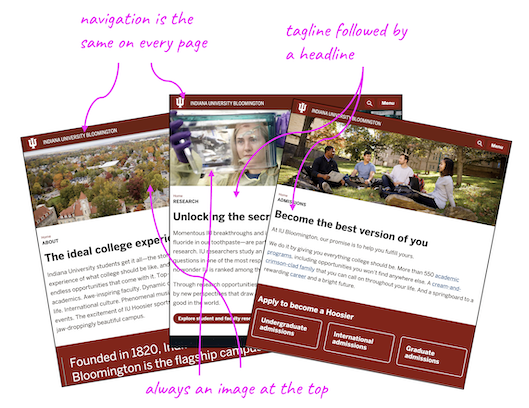
The navigation is repeated on every single page!
Each page contains an image, tagline and headline, with the same styling and in the same order! (though the content in each element is not exactly the same)
Both of these situations can be handled with much less code than in a simple website by using another feature of web applications - templating.
Templating
Remember web applications:
- make use of a database - more on that in Unit 3
- allow us to reuse parts of the code - this is called templating
- provide more control over the URL - this is called routing
In this chapter, let’s focus on templating, meaning we can reuse code for parts of our interface that repeat. (e.g. a navbar)
Templating also allows us to create dynamic websites because we can use Python/Flask to mix and match HTML and content as needed based on user requests. (e.g. the image and headline in the example)
In our web app, the HTML pages will be constructed as templates, and will live in the templates folder:
flaskapp
└── static
└── templates
├── about.html
├── base.html
└── index.html
├── app.py
└── ...
Any HTML pages added to our application should be placed in this folder.
Jinja
Flask makes use of a templating engine designed to work with Python called Jinja.
You’ll notice under the ‘Installation’ section that we use pip to install Jinja, and indeed, we have already done this. Jinja was part of the requirements.txt we used to install the software needed for our Flask web app.
JINJA IS ALREADY INSTALLED!! 👏
Why use Jinja?
Jinja gives us a way to easily reuse code and content by creating placeholders.
You may remember we have a way to make placeholders as f-strings in Python:
story = f"It was a {adj1} and {adj2} {time-of-day}."
In Flask, the Jinja placeholders will help piece together our HTML pages (controlled by app.py) in order to avoid repeating code when possible.
Developer’s sometimes say your code needs to be DRY, which means “Don’t Repeat Yourself”. The goal for this software development principle is to reduce repetitive patterns and limit duplicate code and logic, in favor of modules and code where you can reference the pieces you need only when you need them.
Making our HTML into Jinja templates will DRY our code right out.
How to use Jinja for templating
Several Jinja placeholders (or Jinja calls them ‘delimiters’) are available – we will make the most use of two of these:
- {% … %} for Statements
- {{ … }} for Expressions to print to the template output
The first syntax {% %} is useful for creating placeholder code blocks, or when you need to make use of some basic Python-like functionality like conditional statements (if/else) or loops.
When we say in class “Jinja print”, the second syntax {{ }} is what we are talking about. It’s good for printing out variables, and also for running functions like url_for().
Using Jinja Statements for conditionals and loops
Two basic control structures are essential:
Looping over data with Jinja
<!-- Similar to Python's for loop - 'user' is the key -->
<ul>
{% for user in users %}
<li>{{ user }} : {{ users[user] }}</li>
{% endfor %}
</ul>
Making a decision with Jinja
<!-- Similar to Python's if/else conditionals -->
{% if user == 'admin' %}
Welcome my liege 👑!
{% elif user %}
Access granted.
{% else %}
Access denied.
{% endif %}
Jinja does much more than we will specifically mention in class, and possibly in ways that are more effective or direct. You’ll absolutely want to look through the documentation to see more detailed examples.
Applying Jinja
Let’s now go through the files already present in your templates folder and see how Jinja turns HTML into templates.
base.html
You may have noticed your starter Flask project comes with a base.html.
Open the base.html page and follow along with this next part.
The following HTML tags are required for a page to be considered a web page.
See if you can find these in base.html:
<!DOCTYPE html>
<html lang="en">
<head>
<meta charset="UTF-8">
<meta name="viewport" content="width=device-width, initial-scale=1.0">
<title>{% block title %}{% endblock %}</title>
</head>
<body>
</body>
</html>
In the head, we will be using a Jinja Statement to create a placeholder for our website’s title. Each page may have a different title. Note: this creates a place for a title, but DOES NOT fill in the content.
The code in base.html is code we want repeated on each and every web page in our site.
base.html head
In the head, we will also place any other resources we need for the site to work.
The frontend framework Bootstrap will layout and style our site. Many website resources can be found on a Content Distributed Network (CDN) that provides a link to download the resource when included. That way we don’t have to include the code for that tool in our files. See if you can find the CDN link for Bootstrap.
We also have provided a favicon.ico, which is a little icon that appears next to the name of your site in the browser’s tab.
This is also where you can include any custom stylesheet(s) for your own CSS styles. The one we’ve included is to give users an option for light or dark mode.
base.html body
In the body, we will place any elements that APPEAR IN THE BROWSER WINDOW ON EVERY PAGE.
nav
It’s complicated looking, but we bet you can find the header with a nav nested inside without too much trouble? Find it?
OK. Now notice the unordered list nested inside nav:
<ul class="navbar-nav me-auto mb-2 mb-md-0">
<li class="nav-item">
<a class="nav-link" href="{{ url_for('about') }}">About</a>
</li>
</ul>
Everytime we want to add a new link to our navigation bar, we will add a new li list item like the one we have for the About page.
main
main is where we will be adding all the content for our pages! Notice it contains container that Bootstrap needs for structuring the content, as well as a div with some spacing so our content is positioned better.
<main class="flex-shrink-0">
<div class="container">
<div class="mt-5 pt-5 mb-5">
{% block content %}{% endblock %}
</div>
</div>
</main>
We are adding a placeholder for a block of content using a Jinja Statement. The content block needs both an opening {% block content %} and closing {% endblock %}. No content goes between these placeholder tags in base.html.
footer
The footer in a website is an optional area at the end of the page for information like copyrights, social media, quick links to popular content, directions, and so on. The modern usage for this space is as a kind of catch-all for everything a user might be quickly looking for but didn’t find because here they are at the bottom of the page.
JavaScript
At the very bottom, just before the </body> close body tag, you may also see one more more <script> tags. This is for any JavaScript we want to include on the page. You may also see script tags in the head sometimes too.
index.html
The index page is the home page for a website. It is also our FIRST OPPORTUNITY to fill in the placeholders created in base.html.
In the base template, we made two placeholders — one for a title, and one for a block of content. By EXTENDING this template, we can now create pages that will use all the HTML found in base.html, and then we only need to worry about adding the content specific to the page.
{% extends "base.html" %}
{% block title %}Home{% endblock %}
{% block content %}
<h1 class="display-4">Headline</h1>
<p class="lead mb-5">Opening paragraph.</p>
<!-- more content -->
{% endblock %}
EVERY PAGE YOU MAKE FOR YOUR WEB APP WILL HAVE THESE THREE JINJA STATEMENTS.
- The first extends the base - meaning all the code from the base.html will be loaded first
- The second provides content for the title that appears in the browser tab
- And the third is for any content appearing on that specific page
In general, for the projects we will be building, you’ll want an h1 tag because that is the title appearing at the top of each webpage.
Revisiting about.html
Let’s revisit the route we created for a user wanting to see the About page.
1. The user first clicks on a link in the navigation bar. Because the navigation is found on every page of our web app, the code for the navbar lives in base.html.
<!-- base.html - in the navbar -->
<ul class="navbar-nav me-auto mb-2 mb-md-0">
<li class="nav-item">
<a class="nav-link" href="{{ url_for('render_about') }}">About</a>
</li>
</ul>
The url_for() is wrapped in a Jinja Expression. Flask knows to look in app.py for the about function.
2. Next we go to app.py to run the function about().
# app.py
@app.route('/about')
def render_about():
return render_template('about.html')
The render_template() function is required here to process the Jinja now present in our HTML templates. This function visits the templates directory in our web app, finds the template mentioned, in this case about.html, and sends it on to the browser for display.
flaskapp
└── static
└── templates
├── about.html
├── base.html
└── index.html
├── app.py
└── ...
3. The about.html page is found in the templates directory and displayed in the browser
Practice
Let’s start by updating our About page to make use of Jinja templating. This will improve the look and feel of the content, and allow us to see the power of Jinja. ⚡️
Follow Along with the Instructor
Practice with the instructor. Not an exact replacement for the written directions. You’ll want to work through with me, but also make sure to read the rest or even try again on your own just following the directions.
- Revising the About route, but this time with Bootstrap and templating. Adding CSV data to our web app.
- Updating the Index route (home page) to make use of the data in the CSV and Bootstrap.
Update the About Page to Use Jinja Templating
Add the following code to your about.html page. Replace the ... seen in the title block and content block with the title ‘About’ and the content we already have. Remember the Jinja Statement must wrap around the content. It has a start and end tag just like HTML does.
{% extends "base.html" %}
{% block title %}...{% endblock %}
{% block content %}
...
{% endblock %}
When you’re done, the About page should now display a navigation bar and footer, and updated typography styles.
Update the Home Page (index.html)
Open up index.html and replace the code with the following:
{% extends "base.html" %}
{% block title %}Make This Now{% endblock %}
{% block content %}
<h1 class="display-4">🍳 Make This Now!</h1>
<p class="lead">Simple, delicious recipes to keep you happy
and your belly full.</p>
{% endblock %}
We also need to update the link to the home page in the navigation. Open up base.html and replace the navbar branding line in <header> with this version:
<a class="navbar-brand" href="#">Make This Site Now! 🍳</a>
The link # is just a placeholder. Replace it with the Jinja method for creating a link in a Flask web app.
Solution
href="{{url_for('render_index')}}"
Display Available Recipes on the Home Page
Next, we want to display all available recipes on our home page. We will need to make use of Jinja, routing, Bootstrap, and knowledge of how to read in and unpack a CSV file using Python.
Access a CSV with Recipe Data
1. Add recipes.csv to your project’s root directory. This is OUTSIDE of the flaskapp directory.
root
└── vscode
└── flaskapp
├── venv
├── recipes.csv
└── ...
2. Open app.py, import the csv module, and add the function get_all_recipes():
# Add after 'from Flask...'
import csv
# Add after 'app = Flask(__name__)'
def get_all_recipes():
with open('recipes.csv', encoding='UTF-8-sig') as csvfile:
contents = csv.DictReader(csvfile)
all_recipes = {row['recipe_slug']: {
'recipe_slug': row['recipe_slug'],
'recipe_name': row['recipe_name'],
'description': row['description'],
'recipe_image': row['recipe_image'],
'rating': row['rating'],
'url': row['url']
} for row in contents}
return all_recipes
# all routes are below this code
This function reads in the CSV file recipes.csv, and loads the content as a nested dictionary. That means all_recipes will be a dictionary of dictionaries.
# {slug : {dictionary}, slug: {dictionary}, ...}
{
'Microwave-Mac-and-Cheese': {
'recipe_slug': 'Microwave-Mac-and-Cheese',
'recipe_name': 'Microwave Mac and Cheese',
'description': "This from-scratch mac and cheese cooks in one bowl, and you don't have to boil the macaroni or cook the cheese sauce separately. Plus, it's ready in less than half an hour. A blend of American and Jack cheeses makes the sauce smooth and tangy.",
'recipe_image': 'images/recipe-images/mac-and-cheese.jpg',
'rating': '4',
'url': 'https://www.foodnetwork.com/recipes/food-network-kitchen/microwave-mac-and-cheese-3363099'
},
'5-Ingredient-Chicken-Pesto-Soup': {...},
...
}
Note: A “slug” is a nickname, and usually written without spaces so it can be used as a key like we do here.
Display the Data on the Home Page
Review Routes: Data Out before attempting this next part.
1. Rewrite the root route (“/”) to get all of the recipe data from a CSV and store it in a local variable. Call this variable ‘all_recipes’.
# app.py
@app.route("/")
def index():
# add code here
return render_template("index.html")
2. Now take that variable (set to our nested dictionary of recipes), and pass it out of the route and on to the index.html template page.
Solution: Try it First
@app.route("/") def index(): all_recipes = get_all_recipes() return render_template("index.html", all_recipes=all_recipes)
3. Test that the data made it to the home page. Use a Jinja Expression to display the variable all_recipes on index.html.
{% extends "base.html" %}
{% block title %}Make This Now{% endblock %}
{% block content %}
<h1 class="display-4">🍳 Make This Now!</h1>
<p class="lead">Simple, delicious recipes to keep you happy and your belly full.</p>
# Add your code here
{% endblock %}
Solution: Try it First
{% block content %} ... {{ all_recipes }} {% endblock %}
Never skip this step when setting up a new route. Always make sure the data is present and you understand how it is constructed before attempting to mark it up with HTML.
4. Use Jinja to unpack the data.
The data we’ve brought in is a complex data structure. It’s not just one value, it’s a lot of values. Anything in a list, dictionary, or nested list or dictionary may need to be unpacked so we can see the parts. To do that we need a loop.
Here is the most basic way to write this:
{% for recipe in all_recipes %}
<p>Key: {{recipe}}</p>
<p>Value: {{all_recipes[recipe]}}</p>
{% endfor %}
Notice that ‘recipe’ is the KEY not the VALUE.
Jinja provides several methods for unpacking data using a for loop, but the most straightforward way is perhaps just to use the indexing techniques we already know. Indexing will allow us to access the value for each item in the dictionary just fine.
On this page, we do not need every single aspect of every single recipe. We just need the name and the image. This should show us the data we will need for items on this page:
{% for recipe in all_recipes %}
<p>{{all_recipes[recipe]['recipe_name']}}<br>
{{all_recipes[recipe]['recipe_image']}}</p>
{% endfor %}
Once the data is printing out for each recipe, it’s time to figure out how to improve the design and layout.
5. Use Bootstrap to format each recipe as a card.
We will be using Bootstrap to provide much of the HTML, all of the CSS, and when needed, the JS, in order to focus on what Flask is doing, but still end up with a professional-looking website.
Open the link and look at the first example. This is where the code was copied from, minus a descriptive paragraph and a button, which we don’t need this time.
- Before you get too far with this, go ahead and add this folder of recipe images to your ‘static’ folder under the ‘images’ directory. You’ll need to unzip this resource to use.
On a Mac, and can’t figure out how to find where this project lives on your computer? With the file structure visible (Explorer) in VS Code, right click and “Reveal in Finder”.
Copy in each step below one at a time. Examine the result before moving on to the next step.
First we need the code for a card:
We updated the recipe title to be a H2 in order for the hierarchy to make sense — otherwise the code is the same was what Bootstrap provided.
- H1 “Make This Now!” site title
- H2 Recipe titles
<div class="card" style="width: 18rem;">
<img src="..." class="card-img-top" alt="...">
<div class="card-body">
<h2 class="card-title">Card title</h2>
</div>
</div>
Second, we need to replace the ... and filler text with our content.
Notice that the image is STATIC CONTENT and must be put in accordingly.
{% for recipe in all_recipes %}
<div class="card" style="width: 18rem;">
<img class="card-img-top" src="{{url_for('static', filename=all_recipes[recipe]['recipe_image'])}}"
alt="{{all_recipes[recipe]['recipe_name']}}">
<div class="card-body">
<h2 class="card-title">{{all_recipes[recipe]['recipe_name']}}</h2>
</div>
</div>
{% endfor %}
Third, use Boostrap’s “Grid” to layout the content in rows and columns on the page.
<div class="row">
{% for recipe in all_recipes %}
<div class="col-12 col-md-6 col-lg-4 col-xl-3 mb-5">
<div class="card" style="width: 18rem;">
<img class="card-img-top" src="{{url_for('static', filename=all_recipes[recipe]['recipe_image'])}}"
alt="{{all_recipes[recipe]['recipe_name']}}">
<div class="card-body">
<h2>{{all_recipes[recipe]['recipe_name']}}</h2>
</div>
</div>
</div>
{% endfor %}
</div>
And fourth, also included in the code from step three, the hvr-grow class class to create a rollover effect for each element, and the h-100 class to make the cards all the same height.
<div class="card h-100 hvr-grow" style="width: 18rem;">
Routing and Templating Practice
1. Add a Supplies Page
A user may want to see what supplies we will need in our kitchen to make the recipes posted on our site. This will give us practice with bringing data into our application, and sending that data along the route to the template.
Follow Along with the Instructor
Practice with the instructor. Not an exact replacement for the written directions below.
- Practice with routing and templating, and bringing in data to your app and template, by adding a Supplies page.
SET UP: Download supplies.csv and add to your root directory
root
└── vscode
└── flaskapp
├── venv
├── recipes.csv
├── supplies.csv
└── ...
BEGIN INTERACTION: Add to or adjust the code in base.html to place a link for a “Supplies” page underneath the link for “About”
<nav class="navbar navbar-expand-md navbar-dark fixed-top bg-dark">
...
<ul class="navbar-nav me-auto mb-2 mb-md-0">
<li class="nav-item">
<a class="nav-link" href="{{ url_for('render_about') }}">About</a>
</li>
<!-- Add link to Supplies here -->
CREATE ROUTE: In app.py, add a route called /supplies
The supplies route should:
- have access to a nested list of supplies
- render the template
supplies.html - pass on the nested supplies list to the HTML template
HANDLE DATA: Bring in the supplies list from supplies.csv
Write a function in app.py that reads in supplies.csv as a nested list, where the structure is [[supply-name, description], [], ...].
# place this function near our other open CSV function
def get_all_supplies():
# add code here
return all_supplies
RENDER TEMPLATE: Create a new template page to display all supplies
This HTML template page should:
- have a page title that says “Supplies”
- include required template code
- display the following text:
<h1 class="display-4">Kitchen Supplies</h1>
<p class="lead">To cook the recipes found on this site, you will need a selection of kitchen tools. The following is a list of the essentials.</p>
<!-- Place supplies table here -->
- display the nested supplies list as a table
- supplies table should be styled using Bootstrap (Content > Tables)
2. Add Recipe Details Pages
When we click on a recipe in the home page, the site should open a page with details about that recipe. This will give us practice with writing routes that both require data and pass data along to the HTML template.
Follow Along with the Instructor
Practice with the instructor. Not an exact replacement for the written directions below.
- Practice with routing and templating, and bringing data in and out of your route, by adding a link to a details page for each recipe on the home page.
BEGIN INTERACTION: Add a link to each recipe card on the home page index.html
Add a link around each card, then replace the hashtag # in the link to a new route.
...
<div class="col-12 col-md-6 col-lg-4 col-xl-3 mb-5">
<a href="#">
<div class="card h-100 hvr-grow" style="width: 18rem;">
...
</div>
</a>
</div>
...
CREATE ROUTE: In app.py, add a route called /recipes/<recipe>
The recipes route should:
- have access to the recipe’s slug through the
<recipe>variable - use that slug to find the dictionary for that particular recipe
- render the template
recipe.html - pass on the relevant recipe dictionary to the HTML template
Challenge
- Replace the numeric rating value with a number of ⭐️ instead (hint: copy the star to begin)
Possible Solution: Try it First
one_recipe['rating'] = '⭐️ ' * int(one_recipe['rating'])
RENDER TEMPLATE: Create a new template page recipe.html to display details for a single recipe
This HTML template page should:
- be titled with the name of the recipe
- include required template code
- display the details for the single recipe card clicked on in the home page
- replace the ALL CAPS elements in the code below using Jinja, and as needed, referencing the recipe data pulled into the page
<h1 class="display-4">RECIPE NAME</h1>
<div class="row row-cols-1 row-cols-lg-2">
<div class="col">
<img src="IMAGE SOURCE" class="img-fluid py-3"
alt="RECIPE NAME">
</div>
<div class="col">
<p class="pt-3">RECIPE DESCRIPTION</p>
<p>RECIPE RATING</p>
<div class="d-grid gap-2 d-md-block row-gap-2">
<a href="RECIPE URL" target="_blank" type="button" class="btn btn-primary">Get this Recipe</a>
<a href="LINK TO HOME PAGE" target="_blank" type="button" class="btn btn-secondary">Find Another Recipe</a>
</div>
</div>
</div>
Did you notice? We have 10 recipes, could have more, and yet we have only ONE TEMPLATE that handles all of those pages!
Quiz Yourself: Where is the Data? 🤔
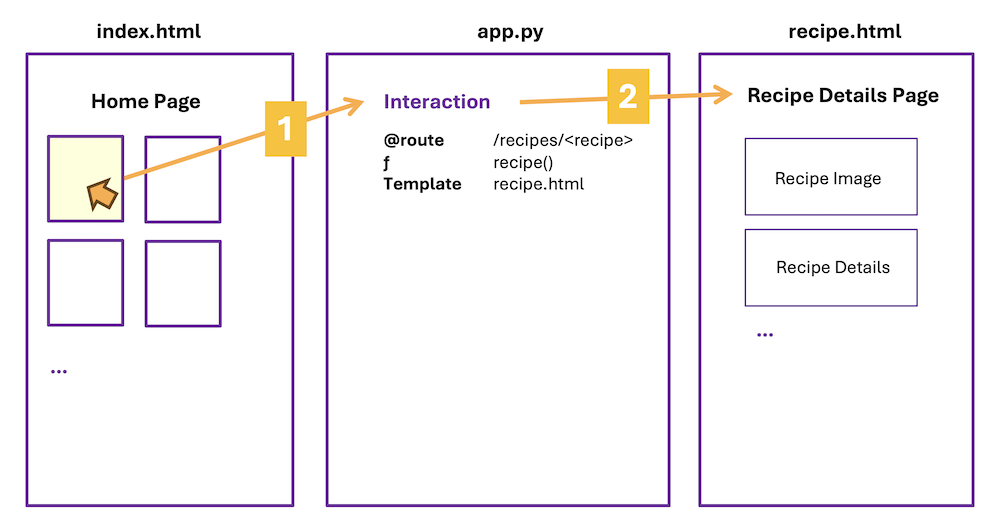
Is data being passed between the start and end of each orange arrow? If so, what is that data? Answer for each arrow:
Interaction 1: Arrow #1
Is data being passed between the user clicking on a recipe in the home page and the function in our route?
Answer to #1
Yes
We need to know which recipe the user clicked on. The route is expecting the "slug" for a recipe. This will become a parameter in our function, and a local variable we can use to look up the details for the recipe clicked on.
Interaction 1: Arrow #2
Is data being passed between the route and the recipe details page?
Answer to #2
Yes
We need to send along the dictionary of data associated with the recipe we clicked on so the page's template can unpack and display the details for this single recipe.
Work Session - v0.2.0
Read the directions for the Project
- View the assignment in Canvas
- Canvas > Modules > Week 3 > What to Do in Week 3
Sketch the interactions
The goal is to sketch each user interaction, indicating pseudo code and access to data along the way.
Let’s try this once together, then you can try the rest of the interactions on your own:
Using pen and a piece of paper, with the paper in landscape, divide the paper into three sections.
- Label the first section index.html
- Label the second section app.py
- Label the third section flowers.html
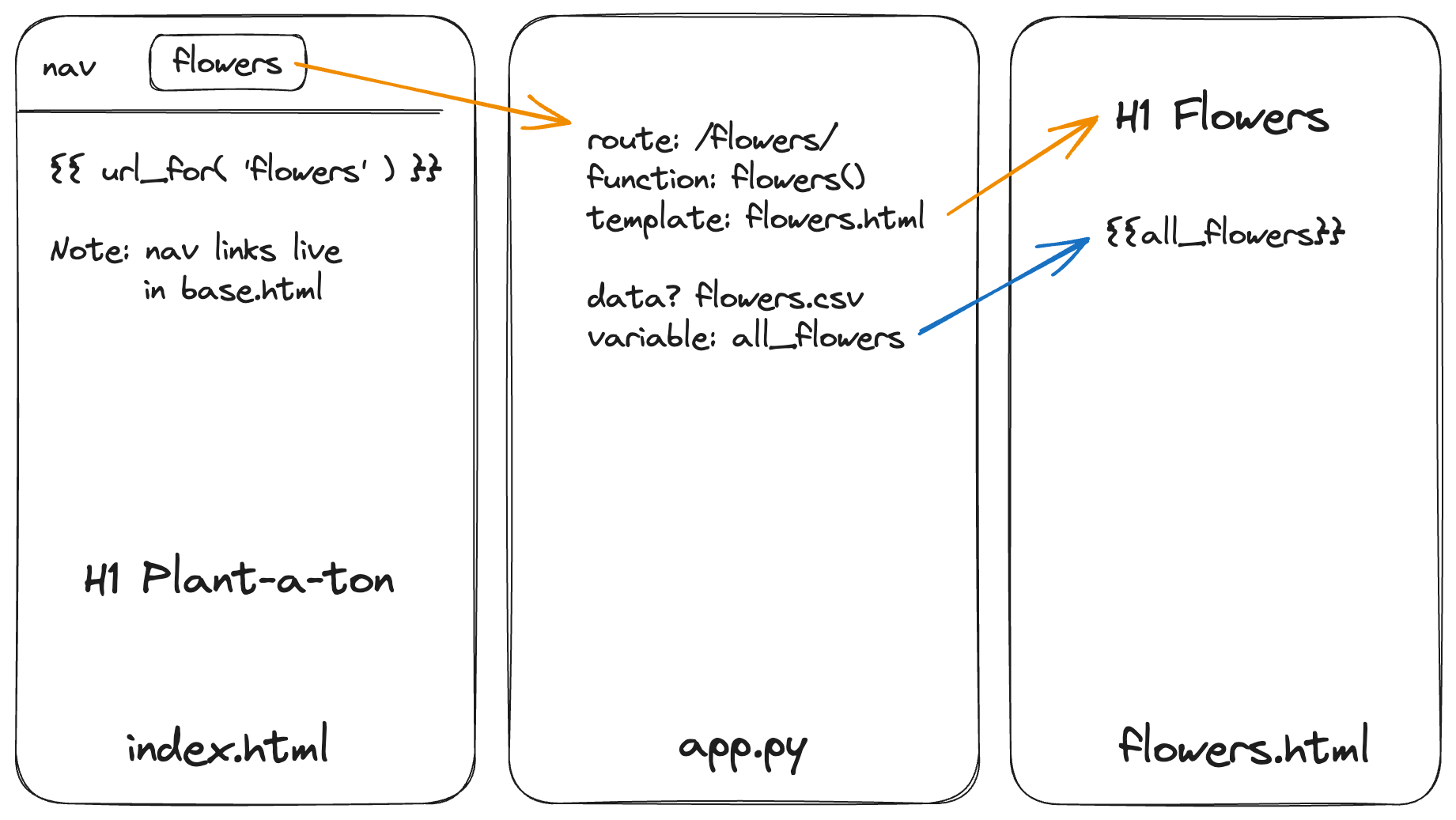
index.html
In the first section, representing index.html, the user clicks on a link in the navigation. Add the link “Flowers” to this column on your page, and add how you would write this link using HTML and Jinja in the template. Do we need to send any data through to the app? If so, indicate that too. (This time, for “Flowers”, we do not.)
Draw an arrow from the link to the middle section representing app.py.
app.py
In the second section app.py indicate:
- Route:
/flowers/ - Function definition:
flowers() - Template to render:
flowers.html - Is there any data coming in? no
- Is there any that needs to be processed or gathered? flowers.csv
- Is there any data to send on to the HTML template? yes, “all_flowers”
Don’t worry about writing the full route code here. We just want to write down the important bits.
Draw an arrow to the final section.
flowers.html
In the third section, representing flowers.html, indicate the variables name(s) for any data passed to the template (all_flowers), and note what the resulting page is for (e.g. it’s the Flowers page)
Repeat this process for each route we have asked you to create. Reference your interaction sketches as you code.
Begin coding
Begin coding for Project v0.2.0, keeping in mind the entire user interaction: from (1) a click on a link, to (2) the route in app.py, to (3) the resulting rendered HTML template.
Forms I - POST and Input
Our web application includes ten recipes, but we promised in the About page that a new feature to add your own recipes was coming soon! Let’s add a page called “Add Recipe” that allows a user to put more recipes on the site.
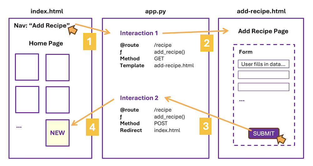
This time we will create a new route that will handle two different user interactions. One to view the template page (Arrows #1 and #2), and one to process the form data. (Arrows #3 and #4) The function for this route will look at the method used to connect with the route, then decide what to do for each scenario.
INTERACTION 1: Create the user pathway to access a new page called “add-recipe.html”
The first user interaction is similar to what we have done so far. When a user clicks on a link in the navigation bar, they should see a page with a form on it for adding recipes.
Follow Along with the Instructor
Practice with the instructor. Not an exact replacement for the written directions below.
- Practice creating the first to two interactions needed to add a recipe to our website.
Add a link in the navigation to “Add a Recipe”
- Links in the navigation live in base.html because they are present on all web pages
- The link should go to the function
add_recipein your routes
Create the route
- The route will be for
/add-recipe - The function is
add_recipe() - The template rendered will be
add-recipe.html
Q: Does this route have any variables we need to handle?
Nope. If it did, it would look more like /add-recipe/
We only need to be concerned with the basics on this route for the moment.
Make an HTML template page called ‘add-recipe.html’
The template page should:
- be placed in the templates folder, and make use of required Jinja template code
- have a page title “Add Recipe”
- contain the following content:
<h1 class="display-4">Add a Recipe</h1>
<p class="lead">Add your favorite recipes to <em>Make This Now!</em></p>
Test this interaction out by running your Flask app before moving to the new interaction. Directions for starting a development server are in the READ.ME.
INTERACTION 2: Creating a form
The first part to creating a form is to add a space for it to live in your HTML code. The start of the interaction is when the user clicks the “Submit” button within the form.
Follow Along with the Instructor
Practice with the instructor. Not an exact replacement for the written directions below.
- Practice creating the first to two interactions needed to add a recipe to our website.
Add a form to add-recipe.html template
Add this code to add-recipe.html:
<!-- add underneath existing text content -->
<form action="{{url_for('add_recipe')}}" method="post" enctype="multipart/form-data">
...
<div class="mt-4">
<button class="btn btn-primary" type="submit">Submit</button>
<button class="btn btn-secondary" type="clear">Clear</button>
</div>
</form>
-
The action attribute in the FORM element uses Jinja to access the route we just created!
-
Method “POST” means that the data should be sent in a more secure method than the standard “GET” method, which is what Flask defaults to when we send data between pages.
-
“Enctype” is set so we are encrypting the data specifically as form data. It’s not absolutely required, but will usually make your form work better and we’d like you to include this option.
-
At the bottom of your form, we have a box with two buttons:
- Submit - when the user clicks this button, the ACTION on the FORM is called
- Clear - when the user clicks this button, the form elements are cleared out, no additional code is required for this to work, and it’s a standard interface option on many forms
This second interaction is kicked off by the user clicking the Submit button, which activates the action set in the FORM element.
DATA: Adding elements to the form
When we want to get data from the user, and not just from an external source like a CSV, we need to create a form that includes a variety of elements designed for collecting data for the user. Open up the documentation and familiarize yourself with what options are available.
See if you can find where Bootstrap talks about the most used types of form elements:
- text input, for anything that is a short piece of text
- text area, for longer sentences or paragraphs of text
- select, which is how you make a dropdown
- checkboxes, for when you want the user to select zero-all options
- radio buttons, for when you want the user to only select one option from many
In the add-recipe form, we will make use of an input (text), textarea, radio button, input (url), and input (file). Notice that three of these are the same type - INPUT!
The input element is flexible that way. It can accept a date, a color, an email, etc.. anything that can be submitted as a short string data type. By specifying, for example, type ‘date’, the INPUT element changes in the interface to pop up a mini calendar for the user. For type ‘email’, the INPUT will do some simple validation to make sure there is an “@” as part of the address.
Structure of form elements
The naming is important. You get to come up with the names, but here are the rules:
-
The for attribute in LABEL and the id attribute in INPUT MUST MATCH - this is how the form knows which label goes with which form element.
-
The name attribute in INPUT becomes the name of the variable when we pull in the form’s data. It is common for this to be the same as ID and FOR, but it can be different.
<div class="mb-3">
<label for="recipe-name" class="form-label">Recipe Name:</label>
<input type="text" class="form-control" name="recipe-name" id="recipe-name" placeholder="Name of Recipe">
</div>
Also helpful to know, a placeholder attribute can be used to give the user an indication of what kind of data is expected.
In general, we want the label and associated form elements to be visually grouped on the page. Notice the DIV with the Bootstrap spacing class on it wrapped around both the LABEL and INPUT.
Add these elements to the form in add-recipe.html
<!-- add to form -->
<div class="mb-3">
<label for="recipe-name" class="form-label">Recipe Name:</label>
<input type="text" class="form-control" name="recipe-name" id="recipe-name" placeholder="Name of Recipe">
</div>
<div class="mb-3">
<label for="description" class="form-label">Brief Description:</label>
<textarea class="form-control" id="description" name="description" rows="3"></textarea>
</div>
<fieldset class="row mb-3">
<legend class="col-form-label col-sm-2 pt-0">Recipe's Rating:</legend>
<div class="col-sm-10">
<div class="form-check form-check-inline">
<input class="form-check-input" type="radio" name="rating" id="rating-1" value="1">
<label class="form-check-label" for="rating-1">
1
</label>
</div>
<div class="form-check form-check-inline">
<input class="form-check-input" type="radio" name="rating" id="rating-2" value="2">
<label class="form-check-label" for="rating-2">
2
</label>
</div>
<div class="form-check form-check-inline">
<input class="form-check-input" type="radio" name="rating" id="rating-3" value="3">
<label class="form-check-label" for="rating-3">
3
</label>
</div>
<div class="form-check form-check-inline">
<input class="form-check-input" type="radio" name="rating" id="rating-4" value="4" checked>
<label class="form-check-label" for="rating-4">
4
</label>
</div>
<div class="form-check form-check-inline">
<input class="form-check-input" type="radio" name="rating" id="rating-5" value="5">
<label class="form-check-label" for="rating-5">
5
</label>
</div>
</div>
</fieldset>
<div class="mb-3">
<label for="url" class="form-label">Full Recipe URL:</label>
<input type="url" class="form-control" name="url" id="url" placeholder="https://www.recipe.com">
</div>
<div>
<label for="recipe-image" class="form-label">Recipe image:</label>
<input type="file" id="recipe-image" name="recipe-image" accept="image/*">
</div>
<!-- this code should be followed by the two buttons and close form tag -->
Take a look at add-recipe.html in a browser to make sure your form looks ok before moving on. You may need to refresh the page to see the updates.
INTERACTION 2: Routing the form’s data
In this second interaction, we begin with the user clicking “Submit”, which activates the form. The form action is set to call the same function we called earlier to view the add recipe page! So we will need a way to decide WHICH INTERACTION is happening when.
Do you recall that the method set in our FORM is “post”?
The logic, then, goes like this:
- If the method is “post” then the user has clicked the “Submit” button in the form.
- If the method is not that, then we just must want to view the add-recipe.html page.
Begin by updating the /add-recipe route:
@app.route("/add-recipe", methods=['GET', 'POST'])
def add_recipe():
if request.method == "POST":
# process the form data, then go to the home page
return redirect(url_for('render_index'))
else:
# view the add recipe page
return render_template("add-recipe.html")
Notice that we are using a new library called request to check the method? We’ll also be using one called redirect soon.
Update the import at the top of app.py in include “redirect” and “request”:
from flask import Flask, render_template, url_for, redirect, request
Update the route to grab the form’s data
To grab the data from the form, we will use request again:
recipe_name = request.form['recipe-name']
recipe_name(with an underscore) is the name of a local Python variablerecipe-name(with a dash) is the name of the name attribute in the HTML form element we want to get the data from
This difference between the underscore and dash seems annoying but it’s meant to help differentiate between your program’s code and the code meant for the interface.
Grab the form’s data and place it into a dictionary
Update the if-statement in add_recipe() to grab the form data:
@app.route("/add-recipe", methods=['GET', 'POST'])
def add_recipe():
if request.method == "POST":
recipe_name = request.form['recipe-name']
recipe_slug = sluggify_recipe_name(recipe_name)
# add variables for the description, rating and url
new_recipe = {
'recipe_slug': recipe_slug,
'recipe_name': recipe_name,
'description': description,
# the recipe image is being set to a default image
# you have this image - it was included in recipe-images (ZIP)
'recipe_image': 'images/recipe-images/null_image.jpg',
'rating': rating,
'url': url
}
# add the new dictionary to our CSV data
return redirect(url_for('render_index'))
else:
return render_template("add-recipe.html")
You’ll also need to add the helper function for the sluggifying 🐌:
def sluggify_recipe_name(name: str) -> str:
"""Convert a recipe name to a "slug" string
Recipe names typically have spaces, which look like %20 in a URL. This
looks terrible, so we will replace the spaces with a hyphen: `-`.
>>> sluggify_recipe_name("Three Bean Chili")
'Three-Bean-Chili'
>>> sluggify_recipe_name("S'mores")
'Smores'
"""
return name.replace(" ", "-").replace("'", "")
Attempt to add the code to grab data from the rest of the form elements on your own first.
Solution to Add the Rest of the Variables
description = request.form['description']
rating = request.form['rating']
url = request.form['url']
We got the data, what’s next?
Getting and then using the data from a form goes like this:
- collect the data together into a dictionary (provided for you)
- add the new dictionary to our CSV data
- redirect to the index page, which will load in the updated CSV data
Note: We put the data into a dictionary for this demo, because the data coming out of our CSV is a dictionary of dictionaries, but it just depends. In some situations a list could be better. In general if you have multiple pieces of data, you’ll want a way to group them together for easier access and to make it easier to pass that information on to the next step – and in Python that means a list or a dictionary.
Add the new data to our CSV
We now need to store the new data along with the rest of our recipe data – and for this demo that means in the recipes.csv.
Add this function under get_all_recipes() to help us with this next step:
def set_all_recipes(all_recipes):
with open('recipes.csv', mode='w', newline='') as csv_file:
writer = csv.DictWriter(csv_file, fieldnames=[
'recipe_slug', 'recipe_name', 'description', 'recipe_image', 'rating', 'url'])
writer.writeheader()
for recipe in all_recipes.values():
writer.writerow(recipe)
See if you can now complete the if-statement (if the method is POST):
- get all of the recipes in our CSV
- add a new item to our nested dictionary, the new item will be the
new_recipedictionary containing the data from the form - set the CSV to be the updated data
Try this out before looking at the solution.
Solution
all_recipes = get_all_recipes()
all_recipes[recipe_name] = new_recipe
set_all_recipes(all_recipes)
Display the results
Since we already have a function that handles grabbing the recipes data and displaying all available recipes on the home page, we don’t need to render a template. We can just redirect the user to the function that is already handling this interaction.
# as found in add_recipe()
return redirect(url_for('render_index'))
Quiz Yourself: Where is the Data? 🤔
Is data being passed between the start and end of each orange arrow? If so, what is that data? Answer for each of the four arrows:
Interaction 1: Arrow #1
Is data being passed between the user clicking on “Add Recipe” in the navigation bar and the “add_recipe()” function in our “/add-recipe” route?
Answer to #1
No
Interaction 1: Arrow #2
Is data being passed between the “add_recipe()” function in our “/add-recipe” route and the template “add-recipe.html”?
Answer to #1
No
Interaction 2: Arrow #3
Is data being passed between the form in “add-recipe.html” and the “/add_recipe” route?
Answer to #3
YES, the data is being passed as POST data, BUT NO, it is not being passed in from the url_for() where the user clicked.
We will use the request library to pull in the data from within the route's function.
Interaction 2: Arrow #4
Is data being passed between the “/add-recipe” route and the home page template “index.html”?
Answer to #4
No. (Not exactly)
We updated the CSV within our route's function, but the index route will pull in the CSV data. No need to pass it along in the url_for().
Forms II - Standardization and Data Types
As both practice and a way to discuss form validation, we’ll add a form for adding a tag to a recipe. This tag will appear on the home page, and also on the details page for each recipe. For example, a recipe with no meat might be tagged “vegetarian”.
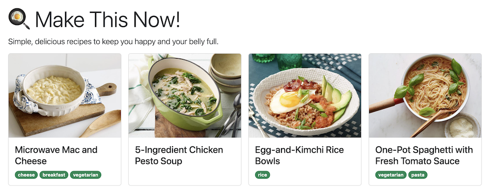
We’ll work with three interactions:
- Updated interaction: pass along new data through the
/recipes/<recipe>route - New interaction: Add tags to the current recipe
- New interaction: Allow the user to create and add their own tags to recipes
INTERACTION 1: index.html to recipe.html using route “/recipes/< recipe>”
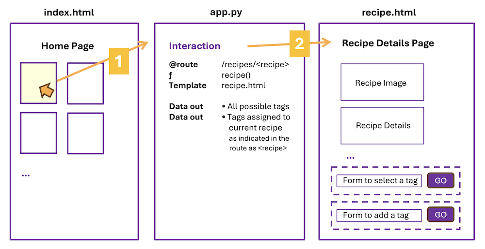
1. Update data available
We will first add the following data to the root directory of your application.
Data showing which tag is attached to which recipe
We could adjust recipes.csv to accept tags, but because a recipe can have more than one tag, it makes sense to have a separate CSV for the tags. This new CSV called tagged.csv has two columns: (1) a recipe that has been tagged and (2) which tag was used. If we added this kind of data to recipes.csv it would have to be in the form of a list, which would then require more work to access.
Data listing all tag possibilities
Next up, we are going to need a list of possible tags. Otherwise our USER can choose and do we really want a tag that says “makes me want to 🤮”? Because that is the tag Erika’s son Max suggested we add. Let’s say we stick to the list we’re giving you for now. 😌
Download tagged.csv and tags.txt and add these files to your file structure:
root
└── vscode
└── flaskapp
├── venv
├── recipes.csv
├── supplies.csv
├── tagged.csv
├── tags.txt
└── ...
Once you place these two data sources into your lecture project, look at the files in VS Code. You’ll have a better idea of what we are working with.
- In tagged.csv, we see two columns of data. A recipe’s name in slug format, followed by the name of the tag.
- In tags.txt, we see possible tags displayed as one string per line.
Note how we are connecting these data sets
Notice that we are referring to recipes in “tagged.csv” by their slug 🐌 and not their recipe name, and that “recipes.csv” also has a slug as part of the data. A consistent way to reference each item in our data will help us connect the two data sets together. (More on this in Unit 3!)
Follow Along with the Instructor
Practice with the instructor. Not an exact replacement for the written directions below.
- Update the recipes route to include tag data.
2. Update the route to pass tagged data to recipe.html
Right now, recipe.html is receiving a dictionary that contains details for a single recipe. We also want this page to have access to the tag-related data we added to our app.
Update your /recipes/<recipe> route to send additional data along to “recipe.html”:
@app.route('/recipes/<recipe>')
def recipe(recipe=None):
all_recipes = get_all_recipes()
if recipe and recipe in all_recipes.keys():
one_recipe = all_recipes[recipe]
one_recipe['rating'] = '⭐️ ' * int(one_recipe['rating'])
return render_template(
'recipe.html',
one_recipe=one_recipe,
tagged_as=csv_to_tbr()[recipe],
all_tags=sorted(get_tags())
)
else:
return redirect(url_for('index'))
In the data being passed along to the recipe.html template by render_template():
- “one_recipe” was there before and passes a dictionary with details about the chosen recipe
- “tagged_as” are the tags from tagged.csv, but ONLY for the current recipe
- “all_tags” is a sorted list of all possible tags (strings)
Notice that we are using some functions you might not recognize. These are helper functions we wrote to manage the tags and tag data.
- “csv_to_tbr” gives us a dictionary where the recipe is the key, and the tag associated with the recipe is the value - notice we are only passing along the tags for the recipe we are going to view
- “get_tags” loads the tags from a text file and creates a list
For your code to actually work, you’ll need to import a new library:
from collections import defaultdict
# add directly above 'import csv' at the top of app.py
Then add these helper functions to app.py:
# add these helper functions near where your other helper functions live in app.py
def get_tags() -> set[str]:
"""Load all tags as a set of strings"""
with open("tags.txt", newline="") as fh:
return set(fh.read().splitlines())
def csv_to_tbr() -> dict[str, set[str]]:
"""Turn a CSV of key-value pairs into a dictionary representing
"tags by recipe", or "what tags does a recipe have?"
i.e.:
by_recipe = {
"Microwave-Mac-and-Cheese": {"vegetarian"},
"One-Pot-Spaghetti-with-Fresh-Tomato-Sauce": {"vegetarian"},
}
"""
# The `defaultdict` is optional here, but using it means we can avoid
# writing a lot of boilerplate. i.e.: If a key is not present in the
# defaultdict(set): the tags are equal to the empty set.
by_recipe = defaultdict(set)
with open("tagged.csv") as csvf:
for row in csv.DictReader(csvf):
by_recipe[row["recipe"]].add(row["tag"])
return by_recipe
Now that two additional pieces of data are being passed along to “recipe.html”, we need to write Jinja to handle them in the template.
Quiz: Test yourself
What are the variable names for the data being passed to the recipe.html page?
one_recipe - dictionary with recipe details
tagged_as - a list of tags applied to current recipe
all_tags - a list of valid tags
3. Update recipe.html to display any tags for the chosen recipe
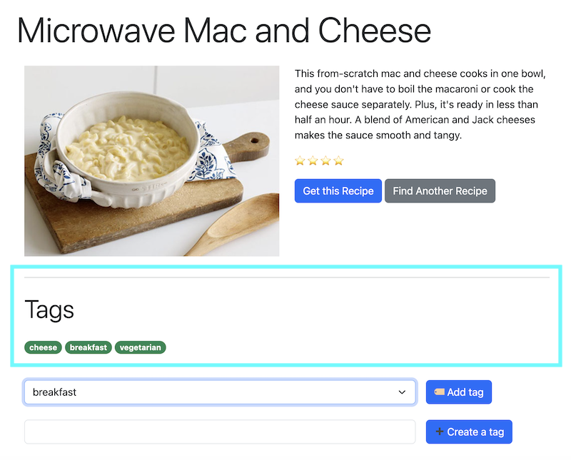
Directly under the HTML content in recipe.html, let’s make space to display tags associated with the current recipe. To display these tags, we will need to access the “tagged_as” data we passed to this page.
<!-- existing code for displaying recipe details -->
<hr>
<h2 class="display-6 my-4">Tags</h2>
{{tagged_as}}
ALWAYS a good idea to “Jinja print” out the data and make sure (1) it shows up and (2) it is the format you expected.
Format the tags
- Using Jinja, display each tag. (Q: What data type is the “tagged_as” data?)
- Use Bootstrap to style each tag:
<span class="badge rounded-pill text-bg-success">PLACE TAG HERE</span>
Solution
{% for tag in tagged_as %}
{{ tag }}
{% endfor %}
Data validation
What if the recipe is not tagged? We also need to make sure that if the tagged data is empty, that we are handling that scenario.
- Use an if-statement in Jinja to display a message such as “No tags yet” if the tagged data is empty
Solution
{% if not tagged_as %}
No tags yet
{% endif %}
Using a conditional to check if the variable is empty, or if data is present, gives us a way to display different HTML depending on the result of that check.
INTERACTION 2: recipe.html to recipe.html using route “/api/tags/< recipe>/add”
In this interaction, the user is able to tag a recipe.
Follow Along with the Instructor
Practice with the instructor. Not an exact replacement for the written directions below.
- Create a route for tagging a recipe from recipe.html.
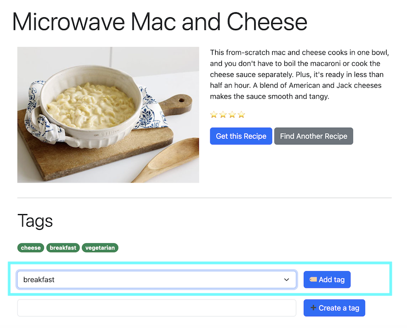
1. Add a form to “tag” a recipe
In the details page for each recipe, let’s add a form for a user to tag a recipe as “vegetarian” or as a meal that’s suitable for “breakfast”.
To begin the interaction, when a user is on the recipe.html page, they can use a simple form to add a tag to the recipe page they are on. This will consist of a dropdown menu (SELECT) and a button.
Start by adding a form to recipe.html underneath the current content:
<!-- Add underneath where the tags are displayed -->
<form action="" method="POST" class="row g-3 my-4">
<div class="col-9">
<select name="tag_name" id="tag_name" class="form-select" aria-label="all available tags">
<!-- Complete this dropdown -->
</select>
</div>
<div class="col-3">
<button type="submit" class="btn btn-primary">🏷️ Add tag</button>
</div>
</form>
- the form action will eventually call a function, but we aren’t ready for that yet - if we add the function before the function is written we will get an error
Data validation: limit choices with a dropdown menu
Another way to improve our code is to make sure the user cannot give us a bogus tag.
- In this form, complete the dropdown to allow users to select from one of the tags available in the
all_tagslist. Use an option/value set up and not just an option please.
Solution
{% for tag in all_tags %}
{% endfor %}
Anytime a user can type into an input, mistakes will be made. By providing only valid options, we can eliminate the user attempting to select a tag that isn’t there.
2. Write a new route to handle a user tagging a recipe
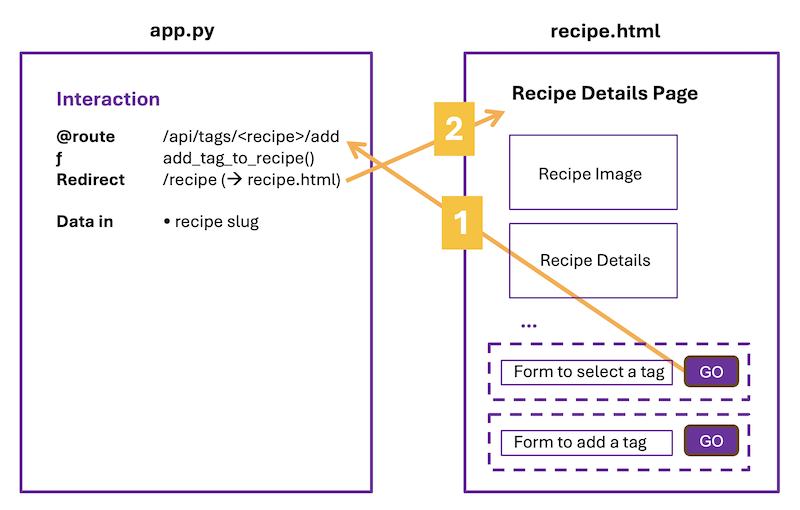
When the user clicks on the “Add Tag” button in recipe.html, the form action calls the function “add_tag_to_recipe()”, and passes along the slug for the current recipe.
First update the form’s action:
<form action="{{ url_for('add_tag_to_recipe', recipe=one_recipe['recipe_slug']) }}" method="POST" class="row g-3 my-4">
- The form action is Jinja brackets around a url_for() calling the function
add_tag_to_recipe. - The url_for() should pass along a variable called ‘recipe’ that contains the visible recipe’s slug (the dashed name for the recipe, and key for our CSV data)
The function add_tag_to_recipe() will:
- grab data form form - only one element “tag-name” in this case
- update the data in the CSV - should now include the tag on the current recipe
- redirect back to see the results - return to the recipe page
Add this new route to app.py:
@app.route("/api/tags/<recipe>/add", methods=["POST"])
def add_tag_to_recipe(recipe: str):
added_tag = request.form["tag_name"]
# get all tagged recipes data from CSV
tbr = csv_to_tbr()
# add the new tag to current recipe
tbr[recipe].add(added_tag)
# update the CSV with new data
tbr_to_csv(tbr)
return redirect(url_for("render_recipe", recipe=recipe))
You’ll also need to add this helper function to app.py for this route to work. It takes a dictionary of tags and updates the CSV with the modified data.
def tbr_to_csv(tbr: dict[str, set[str]]) -> None:
"""Tags-by-Recipe dictionary to a CSV file"""
with open("tagged.csv", "w") as csvf:
writer = csv.DictWriter(csvf, fieldnames=["recipe", "tag"])
writer.writeheader()
for recipe in tbr:
for tag in tbr[recipe]:
writer.writerow(
{
"recipe": recipe,
"tag": tag,
}
)
3. Redirect back to recipe.html to see the result
Once the data has been updated and the new tag (probably) added to the recipe we were on, we want to send the user back to the recipe page to see the result.
@app.route("/api/tags/<recipe>/add", methods=["POST"])
def add_tag_to_recipe(recipe: str):
...
return redirect(url_for("render_recipe", recipe=recipe))
We don’t need to render the template here because we already have a “recipe” route that handles that pathway.
INTERACTION 3: recipe.html to recipe.html using route “/api/tags/< recipe>/add”
In this interaction, the user will type in a new tag to add to the list of possible tags.
Did you notice that interaction 2 and 3 are the same path? Because most of the interaction will be the same, we can use the same route to handle both situations.
Work Along with the Instructor
Practice with the instructor. Not an exact replacement for the written directions below.
- Create a route to let the user add to the list of tags for a recipe.
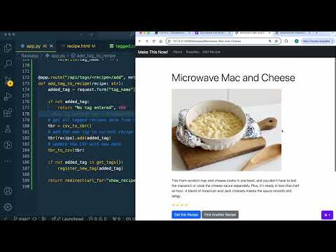
Add a form for a use to enter a new tag

Add this code to recipe.html underneath the current content:
<form action="{{ url_for('add_tag_to_recipe', recipe=one_recipe['recipe_slug']) }}" method="POST" class="row g-3">
<div class="col-9">
<input class="form-control" type="text" name="tag_name" id="tag_name">
</div>
<div class="col-3">
<button type="submit" class="btn btn-primary">➕ Create a tag</button>
</div>
</form>
Route the form to add_tag_to_recipe
NOTICE THAT THE ROUTE AND THE INPUT ELEMENT’S NAME ARE EXACTLY THE SAME!!
All we are doing here is saying instead of choosing from a dropdown, the user can now type in a name instead. We are swapping one way to pass that name along to the route for another. What will change is what we do once we get that tag name.
Add this code to the end of add_tag_to_recipe() just before the redirect:
if not added_tag in get_tags():
register_new_tag(added_tag)
The logic will now look like this:
- if the tag is from our dropdown, we tag the recipe
- if the tag is not from our dropdown, we add it to our list of tags, then tag the recipe
A decision here about whether the tag is included in our list of tags is all it takes to handle both interaction 2 and 3.
For this code to work, you will also need a helper function to add the tag to “tags.txt”:
def register_new_tag(tag_name: str) -> None:
"""Add a new `tag_name` in the set of available tags (i.e. `tags.txt`)"""
with open("tags.txt", "a", newline="") as fh:
fh.write(tag_name + "\n")
What could we improve about adding a new tag?
- We aren’t checking what the user enters AT ALL - they could be entering code to mess with our web app, or adding a couple of unfavorable 🤢🤮😡 emojis!
It’s important to understand that although HTML does provide some validation within form elements, most hackers do not use the interface but instead go directly to your app code.
Ideally, we should validate:
- in the HTML to make the experience better for the user
- in Python/Flask to double check the data coming in from forms, and to make sure that data is valid / clean / not malicious before adding it to our data source (currently a CSV, later on a database).
We have done some simple validation throughout creating the routes to add tags to our app, but clearly we could do more. The first step to knowing what to do is knowing what to ask.
Data validation. Error checking.
What if when we send “recipe” data to “add_tag_to_recipe()” the recipe information is missing, or is not a recipe in our app?
What if when we request the form data from “tag-name”, there is nothing there?
Error checking and validation of data in this function can mean the difference between a program that runs and one that does not. Anytime we work with data coming in from somewhere else, we need to check that it is what we expect, and write code to handle what happens when it is not.
When you test your code, the tests should check for circumstances that mostly don’t happen, but could happen.
Add code to “add_tag_to_recipe()” to check the following:
- is there data for “add_tag”?
- is there data for “recipe”?
- is the recipe a recipe in our recipe data?
You’ll likely need to look at our possible solutions for this, but do think about the approach first. FYI, in our solutions we are returning a “400” status code, which means general error.
Possible Solution
if not added_tag:
return "Bad request, missing tag name", 400
if not recipe:
return "Bad request, missing recipe", 400
if recipe and (recipe not in get_all_recipes()):
return "Bad request, unknown recipe", 400
FINAL STEP: Improve the Recipe Listings
We now have tag data associated with each recipe. The final step is to display tags on the home page as well.
Update the index route in app.py to pass along the new data about tags:
@app.route("/")
def index():
all_recipes = get_all_recipes()
return render_template(
"index.html",
all_recipes=all_recipes,
tags_by_recipe=csv_to_tbr()
)
Note that we already have a helper function to grab all tags from a CSV.
In “index.html” update each recipe to display any tags it may have. Paste the following code inside the DIV with class “card-body” and after the H2 with class “card-title” that is already there:
<p class="card-text">
...
<span class="badge rounded-pill text-bg-success">TAG NAME HERE</span>
...
</p>
Once this code has been pasted in, complete the code:
- use Jinja and the “tags_by_recipe” data to display tags FOR EACH recipe
- note how each tag is represented using Bootstrap
Possible Solution
{{all_recipes[recipe]['recipe_name']}}
{% for tag in tags_by_recipe[recipe] %}
{{ tag }}
{% endfor %}
Using Variables with Jinja
Though not necessary for our lecture app, this technique might help you with the project app!
Sometimes, you want to be able to access part of the data passed from the route to the template, then make a decision. For example, we might need to check if the data came through at all. Or let’s say we want to have all recipes tagged as “cheese” have additional tips for if you want to make the recipes dairy-free (so a CHOICE is involved). Or this can be very helpful when wanting to pre-load data into a form.
Create a Jinja variable
Create a Jinja variable to hold the value:
{% set name = recipe['name'] %}
Then use the variable elsewhere in your HTML template:
<input … value="{{name}}">
In this example, the input has a default value set by a variable. It might be a string, or it might be an empty string if the value is not there.
Additionally, here is a one-line way to do this kind of decision making in Jinja:
<option {% if recipe['name']=="Tomato Soup" %}selected{% endif %} value="tomato_soup">Tomato Soup</option>
In this example, the option appears selected if the data matches the choice.
Or you can even complete this thought in a slightly different way using a more sophisticated Jinja syntax:
<option {{ 'selected' if recipe['name'] == 'Tomato-Soup' else '' }} value="tomato-soup">Tomato Soup</option>
For more Jinja constructions, see the Jinja documentation.
Work Session - v0.3.0
Read the directions for the Project
- View the assignment in Canvas
- Canvas > Modules > Week 4 > What to Do in Week 4
Sketch the interactions
Once again, the goal is to sketch the user interaction, indicating pseudo code and access to data along the way. This time there is still data coming from a CSV, but now we will also focus on what we need from various forms.
Divide a piece of paper into three sections.
- Label the first section gardens.html
- Label the second section app.py
- Label the third section garden-form.html
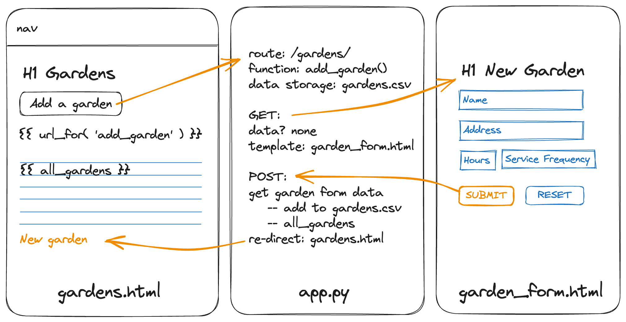
In the first section, the user clicks on a “Add a New Garden” button. Indicate the button and how you would write the link using Jinja. Do we need to send any data through to the app? If so, indicate that too.
Draw an arrow to the middle section.
In the second section, indicate:
- @Route: e.g. gardens/add/
- Function definition: e.g. add_garden()
- Template to render: e.g. garden_form.html
- Any data that needs to be processed, gathered and/or sent on to the HTML page
Don’t worry about writing the code here. Just write down the important bits.
Draw an arrow to the third section. Indicate any data that has been passed to the page, and note what the page is for (e.g. Add Garden page)
Repeat this process for the second half of this route, and for the rest of the routes we have asked you to create. Reference your interaction sketches as you code.
Begin coding
Begin coding, keeping in mind the entire user interaction from a click on a link, to the route in app.py, to the resulting rendered HTML template.
I211 Unit 3: Backend to Database
Welcome to Unit 3! We focused on the front end and back end in Unit 2—and we made the intellectual leaps required for those two views to “talk” to each other. We used a Unix-like file system for state management: storing our pages, images, and data inside of files on the opearting system. But now we have to contend with some limitations of using the file system.
When developers refer to the full stack, as in a “full-stack application” or “I’m a full-stack developer”, what they mean is they have the ability to work on all three layers of a web application.
Now we’re ready to add in that final layer: a database.
In Unit 3
We will:
- add data to a database connected to our web application
- use SQL (Structured Query Language) to make requests and ask questions of that data
- have Python control our SQL requests to the database
- update our Flask application and templates to process and display that data
You will find that once the set up is in place, applying this ‘third layer’ is actually less code and easier to understand and maintain than our previous workflow using a CSV.
CSVs are perfect for bringing data in for display, but they quickly become problematic when we want to change that data, whereas databases are designed for easy access and adjustment of data.
Let’s get started!
Structured Data II: SQL
Are you seeing the limitations of using text files and CSV files yet? They are frequently the simplest and fastest way to get a minimum viable product in front of users: just store and load data from files on the operating system.
But perhaps you’ve also been bitten by one or more of their limitations.
Perhaps you made a mistake when writing to a file. Perhaps you started with a text file that contained data:
$ cat data.txt
1
2
3
… and you wanted to update this file by putting the number 4 after the 3:
>>> with open("data.txt", "w") as fh:
... fh.write("1\n2\n3" + 4 + "\n")
...
Traceback (most recent call last):
File "<stdin>", line 2, in <module>
TypeError: can only concatenate str (not "int") to str
Oops. We made an honest mistake while updating the file. But our honest mistake erased data.txt:
$ cat data.txt
$
Perhaps you were annoyed that everything was a string. Even if there were a column similar to “age” where everything looked like a numeric value:
$ cat turtles.csv
"species","length","age"
"Spotted","5.0 5.0",92
"Spotted","5.1 4.9 5.0",30
… there is nothing in the CSV specification to guarantee this observation, so the default behavior made by Python’s csv standard library (and many similar implementations) is to represent every piece of data as a string:
import csv
from pprint import pprint
with open("turtles.csv") as csvf:
pprint(list(csv.DictReader(csvf)))
$ python3 stringly_typed.py
[{'age': '92', 'length': '5.0 5.0', 'species': 'Spotted'},
{'age': '30', 'length': '5.1 4.9 5.0', 'species': 'Spotted'}]
Perhaps you noticed we had to save and load the whole file every time. When we wanted to modify a single row in a CSV file, we showed that we had to load the entire thing, perhaps with Python’s csv.DictReader, update it, and write it back out with csv.DictWriter:
import csv
# Read the *entire* dataset into Python
with open("turtles.csv") as csvf:
data = list(csv.DictReader(csvf))
# Write the *entire* list-of-dictionaries back to a file
with open("turtles.csv", "w") as csvf:
writer = csv.DictWriter(csvf, fieldnames=["age", "length", "species"])
writer.writeheader()
writer.writerows(data)
… for tiny datasets this isn’t necessarily a problem. But what if our file was 10× bigger? or 100× bigger? Our application would become slower proportional to how big our files were. But what if our data was 100 gigabytes and did not fit in our computer’s main memory?
Data storage guarantees, data types, and partitioning data into logical groups are some of the guarantees that a database provides. A database is a program providing a standardized way to store and query data. Many types of databases exist, each specialized to handle the data storage and querying needs of particular groups of people (a few off the top of Alexander’s head: NoSQL, graph databases, vector stores, search engines, blob storage, key-value stores).
In other words—for any problem that you can imagine, there is an implicit data storage and data management problem. We will avoid most of these choices and complexities (they are topics for another course). Instead we will focus on three types of data modeling approaches. We’ve already encountered two of them:
- Hierarchical data or tree-structured data, which is how we represented file system and the object references used in many programming languages.
- Graph data, which is how we described the structure of the Internet and other means of human communication.
There is one final idea that we want to cover as we draw near the conclusion of this course. When Edgar F. Codd proposed the relational model in 1970,1 he invented it specifically as a way to counter problems that arise when storing data using the previous two approaches.
- Relational data, where data are represented as discrete sets of items, and relations between items.
This idea: storing databases of tuples and relations has proved invaluable for the last fifty years. The relational model, relational databases based on the relational model, and the relational database management systems (RDBMS) comprised of the former.
Today we:
- introduce the relational model,
- its implementation in the MariaDB RDBMS, and
- its creation and querying with structured query language (SQL).
Follow Along with the Instructor
Not an exacty replacement for the book, but let’s highlight some major points together and introduce the relational model.
From tabular to relational data
Edgar F. Codd proposed the relational model in 1970 while working as a programmer at IBM.1 The key ideas were derived from set theory, tuples, and relations defined on related sets of tuples.
Remember how we began the CSV chapter with an example where we were buying groceries for Alice and Bob?
| name | aisle | for |
|---|---|---|
| milk | 24 | Bob |
| cheese | 23 | Bob |
| eggs | 19 | Alice |
| chicken noodle soup | 6 | Alice |
| chicken noodle soup | 6 | Bob |
Now imagine that we also had to represent other information about the people that we were shopping for. Alice and Bob probably have phone numbers and addresses:
('Alice', '123-1122', '123 Street Ave.')
('Bob', '113-7812', '124 Avenue St.')
How would we put data about their phone numbers and addresses into the existing table? We could add new columns for phone numbers and addresses, but now we’ve effectively duplicated our data. Every time we see the name “Alice” or “Bob” have to copy their phone number and address into that row:
| name | aisle | for | phone | address |
|---|---|---|---|---|
| milk | 24 | Bob | 113-… | 124 Av… |
| cheese | 23 | Bob | 113-… | 124 Av… |
| eggs | 19 | Alice | 123-… | 123 St… |
| chicken noodle soup | 6 | Alice | 123-… | 123 St… |
| chicken noodle soup | 6 | Bob | 113-… | 124 Av… |
This exacerbates an earlier problem: we have multiple “chicken noodle soup” rows, and multiple “people” rows. If we had to update this data at a later point in time, we’d have to be mindful of all the places we’ve copy-and-pasted the data and make sure we change them in every single location.
We’ll call this a data normalization problem in a bit. The relational model would propose that instead of the flat tabular data representation, we could instead model the three concepts underlying our problem:
- people: with names, phone numbers, and addresses
- groceries: which are located on a particular aisle
- orders: which people want which groceries?
Rather than trying to force these facts into one giant table, we could instead split them into three smaller tables that each focus on a particular part of our data:
| person | phone | address |
|---|---|---|
| Bob | 113-… | 124 Av… |
| Alice | 123-… | 123 St… |
| name | aisle |
|---|---|
| milk | 24 |
| cheese | 23 |
| eggs | 19 |
| chicken noodle soup | 6 |
| name | for |
|---|---|
| milk | Bob |
| cheese | Bob |
| eggs | Alice |
| chicken noodle soup | Alice |
| chicken noodle soup | Bob |
Each table represents a relation. Each column represents an attribute of that relation, and the total number of columns in a table corresponds to the relation’s arity (binary, ternary, etc.). These concepts provide an abstraction: a higher-level representation of how data are stored and eventually queried. One could look at a high-level picture of the data, such as is shown in an entity-relationship diagram,2 without needing to see every tuple. We decomposed the giant table into a series of relations between attributes: “people place orders”, “an order contains groceries”:
erDiagram
PERSON {
string name
string phone
string address
}
GROCERY {
string name
int aisle
}
GROCERY }o--o{ ORDER : containing
PERSON }o--o{ ORDER : places
This decomposition is closely related to what Codd and others call data normalization. The precise nature of normalization requires several other concepts. Briefly: what would happen if there were two people who were named Alice?
| person | phone | address |
|---|---|---|
| Bob | 113-… | 124 Av… |
| Alice | 123-… | 123 St… |
| Alice | 112-… | 125 St… |
We previously assumed that every name was unique. Therefore when we kept track of each person’s order we put in their name and the item they wanted. But if there were two people named “Alice”, we can no longer look at this entry and know who an order belongs to:
| name | for |
|---|---|
| … | … |
| eggs | Alice |
| chicken noodle soup | Alice |
| … | … |
Codd introduced this as a problem of cross-referencing data between two relations, but also showed there was a “a user-oriented means” of fixing this: unique identifiers called keys which could reference individual pieces of data. Keys came in two varieties: primary keys that uniquely identify each piece of data, and foreign keys which refer to or reference keys inside other relations.
In our person table, we can introduce an id attribute. Identifier attributes that uniquely identify every piece of data rarely occur naturally. Here we will invent an identifier, a primary key integer that starts at 1 and increments every time we need a new person:
| id | person | phone | address |
|---|---|---|---|
| 1 | Bob | 113-… | 124 Av… |
| 2 | Alice | 123-… | 123 St… |
| 3 | Alice | 112-… | 125 St… |
Now we can replace everywhere that previously referred to the first Alice with her foreign key: 2 referencing the id attribute in our other table:
| name | for |
|---|---|
| … | … |
| eggs | 2 |
| chicken noodle soup | 2 |
| … | … |
Now we’re ready for an imperfect but nevertheless good-enough definition of normalization: a fully normalized3 data set is one without redundancy, where every row which can be uniquely identified is uniquely identified, and when we need to cross reference data we do so through primary and foreign keys. Normalized data is often useful: if we need to change something then we only need to change it in one location, as opposed to that giant CSV we started with where changing a person’s address would require updating multiple rows of data.
So far our discussion is high-level and theoretical. In reality: we have to deal with questions like: Where does data come from? How do we define a relation? How do we add or remove data over time? We’re ready to interact with an implementation of the theoretical model: in the MariaDB database.
MariaDB
There are many variants of relational databases to choose from, just like there are many flavors of Linux available. If you’ve heard of any of them, you’ve likely heard of Oracle, MySQL, or Microsoft SQL Server. In Informatics, we use MariaDB, which is a fully open-source variant of MySQL.
Log into MariaDB. Begin by logging into the SICE server “SILO” using your IU credentials:
ssh USERNAME@silo.luddy.indiana.edu
You should see a starred banner. From the command line when logged into Silo, we can additionally access the database accounts set up for us:
mysql -h HOST -u USERNAME --password=PASSWORD -D DATABASE
HOST, USERNAME and DATABASE are replaced by your own credentials.
SICE has set an account up for you. These credentials are available in Canvas - see the current week’s page.
$ mysql -h HOST -u USERNAME --password=PASSWORD -D DATABASE
Welcome to the MariaDB monitor. Commands end with ; or \g.
Your MariaDB connection id is 171566
Server version: 10.6.18-MariaDB-0ubuntu0.22.04.1 Ubuntu 22.04
Copyright (c) 2000, 2018, Oracle, MariaDB Corporation Ab and others.
Type 'help;' or '\h' for help. Type '\c' to clear the current input statement.
MariaDB [USERNAME]>
Notice that the command line prompt indicates whether you are local (on your own computer), logged into the Silo server, or logged into the MariaDB through that server.
Follow Along with the Instructor
Again, not an exact replacement for the book, or vice versa. Practice with the examples in the book, then the video demonstrates how Alexander interacts with MariaDB.
Database Terminology
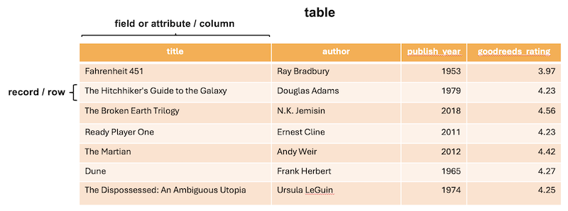
- table: A table is a collection of related data organized into rows and columns
- record: Each row in a table
- field or attribute: Each column in a table
- schema: the logical structure or design that defines how data is organized and stored in the database
Think of this last term, “schema”, as a blueprint outlining the relationships between tables and the data within them. There are lots of flow chart systems for organizing databases in order to indicate relationships between the data tables, what data and methods are included, and so on. Like with a camera, the best one is the one you’ll use.
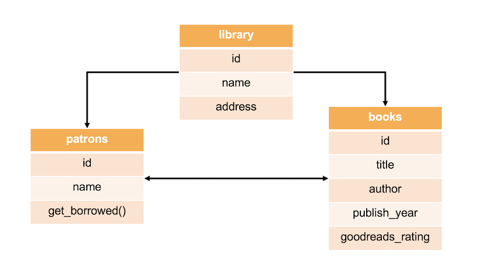
Technically a database can have just one table, but just like with functions in Python, it’s often clearer and easier to maintain if each table has one purpose. We can then build relationships between the tables as we discussed.
Structured Query Language
Information is accessed and modified in a relational database using Structured Query Language (SQL).
SQL is a declarative language, rather than a procedural language like Python. In Python we have to write code that tells the computer exactly what we want it to do (we give directions). In SQL we tell the database what we want from it and the database figures out how to give us the information we want (we ask questions).
SQL is used to ASK QUESTIONS:
You can use SQL to ask questions (“to query”) about the data and it will respond by SELECTING any data relevant to the question.
For example, I might want to know “all students at IU who are Informatics majors”. Or get a list of “all juniors at SICE who are studying abroad in the Spring semester”.
SQL is used to EXECUTE A STATEMENT:
You can use SQL to make specific modifications to the database structure and to the data within. For example, SQL allows you to INSERT, UPDATE, MODIFY data or CREATE, DELETE, ALTER a data table.
Perhaps I need to UPDATE the record for an Informatics student named “Jackie Jackson” to show they have completed all core requirements.
Syntax
The convention in SQL is to CAPITALIZE any of the commands or keywords used, however the SQL will run just fine in lowercase too. (The more SQL you write, the less likely you are to want to type all caps…)
SHOW TABLES;
show tables;
In our examples in your book, we will make use of this CAPITALIZATION convention to help you better understand how SQL queries are constructed. If we need to indicate a variable, something you will fill in, we’ll borrow from the convention used in Flask routes, and use pointy brackets <variable>:
DESC <tablename>;
Finally, notice that all SQL commands typed in on a command line end with a semicolon ; and one common mistake when starting out with SQL, just like in CSS and JS actually, is to forget that semicolon. SQL statements can also be written on multiple lines to make them easier to parse with our eyes. As long as that semicolon is at the end, the new lines are ignored when the statement is executed.
If the cursor hangs after you hit Return when entering a SQL command, it may just be waiting for you to type in a semicolon!
Create a table
CREATE TABLE <tablename> (
<attribute1name> datatype(size) [constraints],
<attribute2name> datatype(size) [constraints],
<attribute3name> datatype(size) [constraints]
) ENGINE=INNODB;
- Commas are used to separate attributes, but not end a list of them
ENGINE=INNOBis enforces referential integrity, basically it’s there to help us- Attribute names (column names), like variables, are case-sensitive. “FirstName”, for example, is NOT the same as “firstname”.
- Datatypes are required by SQL, note that some may also need a size indicated
- Constraints are optional, but often useful
Setting Datatypes
Each attribute (column) in a data table requires not only a name, but also a type for the data. Some choices are more common than others; we’ve listed ones you may encounter in your project.
Datatypes that store character or text data (such as names):
VARCHAR(maxsize)
Variable length character data with a maximum size of “maxsize” characters. Used when we don’t know how long the data is i.e. for first_name, title of a book, phone numbers because these often include non-numeric characters, etc.. this is a very commonly used datatype.
-- Erika Lee, Alexander Hayes, Michal Gordon
-- +1 812-855-6789
first_name VARCHAR(30)
phone VARCHAR(15)
email VARCHAR(50)
The length is up to you, but you want it to be long enough to cover the longest possible possibility for that data. So it’s okay to go a little longer than what you think you might need.
CHAR(fixedsize)
Fixed-length character data of size “fixedsize” characters. Used when we know exactly how long the data is.
-- IN, WI, NV, MD, etc..
state_abbr CHAR(2)
Datatypes that store larger amounts of character or text data:
TINYTEXT
Holds up to 255 characters. Good for text / character data that is several sentences long, like a short description of a book or a short social media post.
-- "I need to buy new window blinds, but I hate dealing with shady salespeople."
social_post TINYTEXT
TEXT
Holds a string of text up to 65,535 characters in length. Good for things like short books or chapters, memos, emails, longer posts, articles, etc…
-- "Unix-like Environments (sometimes written “*nix environments”) refer to ..."
chapter TEXT
Datatypes we use to store numeric data (such as price or quantity):
INT or INTEGER(size) and also FLOAT
Allocates 4 bytes to store a whole number if no size is specified (-2147483648 to 2147483647 for signed numbers, 0 to 4294967295 if unsigned). If specified, “size” is the number of digits.
-- 19, 1000000000, 6.5
age INT,
population INTEGER(10),
shoe_size FLOAT
DEC or DECIMAL(precision, scale)
Allocates precision number of digits with scale decimal places.
- Decimal(5,3) = ± 99.999
- Decimal(7,2) = ± 99,999.99
-- 873.54
price DEC(10,2)
Datatypes to store time and date data:
-- '2024-07-04', '19:30:00', '2024-07-04 19:30:00', '2024'
current_date DATE,
current_time TIME,
current_timestamp DATETIME,
current_year YEAR
DATE
Stores year, month, day in ‘YYYY-MM-DD’ format.
TIME
Stores hour, minute, second in ‘HH:MM:SS’ format.
DATETIME
Stores year, month, day, hour, minute, and second. Uses ‘YYYY-MM-DD HH:MM:SS’ format
YEAR
Stores the year as 4 digits.
We can also add optional constraints to our attributes:
CREATE TABLE students (
id INT AUTO_INCREMENT PRIMARY KEY,
name VARCHAR(50) NOT NULL
);
NOT NULL
Indicates that this attribute cannot have a null (empty) value. Any data inserted into this table must have a specified value for this attribute. Can be used for any attribute.
AUTO_INCREMENT
Used with an INT or INTEGER attribute. Automatically increments the value in the field each time a new record is added. Only one column in a table may be marked with this constraint. Used primarily for ID attributes.
PRIMARY KEY
This unique, not null (not empty) value is how we identify each unique record in our data. It is often an integer, because that makes indexing simple, but doesn’t have to be. The first column in each table will be a primary key. (In i211, we will make these integers.)
Remember, this ability to set a primary key for each record in a table is a step up from using part of the record as the identifier. (What if we are identifying people by name and we had two Alexander Hayes?? 😱) How do we know for sure we are interacting with the right person? A unique ID helps solve that problem.
Create a books table
Let’s write the SQL to create a table called books to hold data with the following types:
- unique
idnumber used as the primary key (and auto incremented) - required
title(up to 255 characters) - required
author(up to 100 characters) publish_yearthat holds a yeargoodreads_ratingstored as a decimal number with 3 digits and 2 decimal places
CREATE TABLE books (
id INT AUTO_INCREMENT PRIMARY KEY,
title VARCHAR(255) NOT NULL,
author VARCHAR(100) NOT NULL,
publish_year YEAR,
goodreads_rating DECIMAL(3,2)
);
Getting Information About a Database
SQL lets us check our how many data tables we have:
SHOW TABLES;
We can also see what attributes (columns) a table contains:
DESC <tablename>;
What this interaction looks like:
MariaDB [i211u24_ebigalee]> CREATE TABLE books (
-> id INT AUTO_INCREMENT PRIMARY KEY,
-> title VARCHAR(255) NOT NULL,
-> author VARCHAR(100) NOT NULL,
-> publish_year YEAR,
-> goodreads_rating DECIMAL(3,2)
-> );
Query OK, 0 rows affected (0.033 sec)
MariaDB [i211u24_ebigalee]> SHOW TABLES;
+----------------------------+
| Tables_in_i211u24_ebigalee |
+----------------------------+
| books |
+----------------------------+
1 row in set (0.001 sec)
MariaDB [i211u24_ebigalee]> DESC books;
+------------------+--------------+------+-----+---------+----------------+
| Field | Type | Null | Key | Default | Extra |
+------------------+--------------+------+-----+---------+----------------+
| id | int(11) | NO | PRI | NULL | auto_increment |
| title | varchar(255) | NO | | NULL | |
| author | varchar(100) | NO | | NULL | |
| publish_year | year(4) | YES | | NULL | |
| goodreads_rating | decimal(3,2) | YES | | NULL | |
+------------------+--------------+------+-----+---------+----------------+
5 rows in set (0.001 sec)
Modifying a table
Right now, we have a table set up, but no data within the table. To add data, and otherwise manage that information, we need SQL to execute statements that modify the table.
NOTE: Once we run a query to make changes in SQL the changes are PERMANENT until you run a query to change things again. You do not need to “save” anything before you log out.
Drop a table
It’s possible to delete a table. If our table has data inside, that data will be deleted as well. Feel free to drop and re-add the books table for practice.
DROP TABLE <tablename>;
Alter a table
We can also make changes to the structure of our tables without necessarily dropping them.
If we forgot an attribute entirely, we can fix that by adding a new attribute:
ALTER TABLE <tablename> ADD <attributename> <datatype> <constraints>;
<tablename>is the table’s name<attributename>is the name of the attribute we want to change<datatype>is the new datatype we want for<attributename><constraints>are any optional constraints we want<attributename>to have
Let’s ALTER our books table to include an attribute for a genre. “COLUMN” is optional here. Run the following commands and after each, use DESC books; to see the alterations.
ALTER TABLE books
ADD COLUMN genre VARCHAR(50);
What if we had added an ISBN and made it the wrong datatype? We can ADD it:
ALTER TABLE books
ADD COLUMN isbn TINYTEXT;
If we messed up and gave the wrong datatype to one of our attributes, we can fix that using MODIFY:
ALTER TABLE books
MODIFY COLUMN isbn INT;
We can also drop/delete an attribute completely using DROP. Let’s go ahead and DROP the columns “genre” and “isbn” for now.
ALTER TABLE books DROP COLUMN genre;
ALTER TABLE books DROP COLUMN isbn;
Putting the data into data tables
Now that our structure is set up, we can use SQL to INSERT, UPDATE, SELECT or DELETE the data within:
INSERT INTO
To add data to any table, we’ll make use of INSERT:
INSERT INTO <tablename> (<attributes>,) VALUES (<values>)[,()] ;
<tablename>is the table’s name<attributes>are the column or attribute names separated by commas<values>are the values for those attribute names in the order they appear
When listing values, use single or double quotes around everything except numbers.
INSERT INTO books (title, author, publish_year, goodreads_rating)
VALUES ('Fahrenheit 451', 'Ray Bradbury', 1953, 3.97);
We can also add multiple lines of data at once:
INSERT INTO books (title, author, publish_year, goodreads_rating)
VALUES ('Dune', 'Frank Herbert', 1965, 4.27),
('The Dispossessed: An Ambiguous Utopia', 'Ursula LeGuin', 1974, 4.25);
INSERT the rest of the data into books either line by line or in multiple lines. When working with MariaDB on the command line, it can be useful to type in the SQL into a blank file, for example books.sql, and then copying and pasting at the prompt to run. It’s easy to make mistakes with commands this long.
'The Hitchhiker's Guide to the Galaxy', 'Douglas Adams', 1979, 4.23
'The Broken Earth Trilogy', 'N.K. Jemisin', 2018, 4.56
'Ready Player One', 'Ernest Cline', 2011, 4.23
'The Martian', 'Andy Weir', 2012, 4.42
With a little pattern matching, this can make adding data fairly straightforward.
Solution
INSERT INTO books (title, author, publish_year, goodreads_rating)
VALUES
('The Hitchhiker''s Guide to the Galaxy', 'Douglas Adams', 1979, 4.23),
('The Broken Earth Trilogy', 'N.K. Jemisin', 2018, 4.56),
('Ready Player One', 'Ernest Cline', 2011, 4.23),
('The Martian', 'Andy Weir', 2012, 2.32);
UPDATE
We can update data in any table in the relational database using the query “UPDATE … SET … WHERE …;”
UPDATE table
SET <attribute> = <newvalue>
[WHERE conditions] ;
The rating for 🛸 The Martian is too low. Let’s UPDATE that rating to “4.42”:
UPDATE books
SET goodreads_rating = 4.42
WHERE title = 'The Martian';
Without the WHERE to add the condition saying to update the rating only for a single title, we would have updated all ratings to be “4.42”. The WHERE narrows where the UPDATE is SET.
SELECT
SQL can also be used to ask questions of the data. We can select all of the data within the table. The basic SELECT query has 3 components to it:
SELECT <attributes we want to return/display separated by commas>
FROM <what table we will be querying>
WHERE <propositional logic conditionals that determine what gets displayed>
We can select all of the data if we want to, using * as a wildcard meaning “all”:
SELECT * FROM books;
The WHERE clause is optional. If omitted, the query will show ALL of the selected attributes from the table.
This means setting WHERE allows us to filter the data coming in from our SELECT. Being more precise with your query is especially useful when working with large datasets. We might want all of the data if we have 10 records, but what if we have 100000000? Returning a lot of records quickly can become slow, or at least not be all that helpful.
What if we just need to know something in particular about the data? Like who the author is for the book “Ready Player One”?
SELECT author
FROM books
WHERE title LIKE 'Ready Player One';
We can use % as a wildcard character to say things like “Select the author for the book where the title INCLUDES the word ‘Earth’”:
SELECT author
FROM books
WHERE title LIKE '%Earth%';
And because SQL understands that data set to be integers or dates can have math applied, we can ask questions like “Which of these books were written after the year 2000?”:
SELECT title
FROM books
WHERE publish_year > 2000;
Or “Which titles have a rating that’s less than 4.0?”
SELECT title
FROM books
WHERE goodreads_rating < 4.0;
Any math comparison will work on dates and numbers, including <= and >= and =.
We can even select both the “title” and “author” from a range of dates, using BETWEEN which also makes use of ‘AND’:
SELECT title, author
FROM books
WHERE publish_year BETWEEN 1950 AND 2000;
Other logical operators:
ORwill return true if either of the two conditions surrounding it is trueNOTwill return true if the condition is false, allowing us to use what we don’t want to select what we do
SELECT * FROM books
WHERE goodreads_rating = 4.25 OR goodreads_rating = 4.27;
SELECT * FROM books
WHERE NOT (title = 'The Martian');
We can also adjust how the information is returned and sort it as ASC ascending or DESC descending.
This is especially helpful for numeric data, and may or may not be what you expect alphabetically because the sorting is done by ASCII code. That means upper- and lowercase letters have different codes and the result may not be what you expect.
Run some examples similar to these to see what we mean:
SELECT title
FROM books
ORDER BY goodreads_ranking ASC;
SELECT author
FROM books
ORDER BY author DESC;
DELETE
And finally, we can delete a row of data from a table using the “DELETE FROM … WHERE …;” statement.
DELETE FROM table [WHERE conditions];
To DELETE the record for the title “Ready Player One”:
DELETE FROM books
WHERE title = 'Ready Player One';
Be careful with this. If your query isn’t written as you expect, you might end up deleting data you weren’t ready to delete. Best to select first and make sure you have the conditions right.
Summary
- We now have the ability to connect to a relational database
- The first step to a good database is to understand the data we want to structure and make a plan for how the tables and the data in them will interact - this skill is a focus for other courses
- Data tables can be CREATE(d) with attributes (with specified datatypes), or we might want to DELETE or ALTER
- Structured Query Language (SQL) also helps us INSERT, UPDATE or MODIFY data in data tables
- SQL is really great at asking questions of data so we can make specific SELECT(ions)
What we need next is an upgrade to our process such that SQL can be used to interact with a database FROM WITHIN our Flask application. We’ll do this using a Python library called PyMySQL.
Want more practice with SQL?
Footnotes
E. F. Codd. 1970. A relational model of data for large shared data banks. Commun. ACM 13, 6 (June 1970), 377–387. https://doi.org/10.1145/362384.362685
Peter Pin-Shan Chen. 1976. The entity-relationship model—toward a unified view of data. ACM Trans. Database Syst. 1, 1 (March 1976), 9–36. https://doi.org/10.1145/320434.320440
We use the phrase “fully normalized” intentionally here, as the version of normalization described by Codd in 1970 is what we now refer to as “First normal form” (or 1NF). The existence of the phrase “first normal form” implies the existence of 2nd, 3rd, 4th, and many other normal forms. These are of theoretical and some practical interest, but we do not want to spend much time on this point. On first glance: people often assume that goals like “remove redundancy” are critical, but in practice: some redundancy often exists for performance reasons. The theoretical guarantees of normal forms are helpful, but in practice: it means actual database systems have to chase foreign keys and spend more time “figuring out” where data is actually stored. “Denormalization” is therefore a trick to squeeze better performance out of systems.
PyMySQL and database connectors
Previously we introduced an interactive approach to working with a database. We (1) opened a terminal, (2) connected to a database, and (3) typed SQL statements and saw the results in real time.
Notice how similar this interactive database REPL is compared to the way we introduced Python. When we introduced Python, we (1) opened a terminal, (2) started the Python REPL, and (3) typed Python statements and saw the results in real time.
Each of these are excellent tools for rapid prototyping: and they should absolutely be used when one is exploring a new idea, or looking up a result. But the day-to-day tasks of a business analyst or data scientist are rarely achieved by typing one-off SQL statements into a REPL then telling people what they saw. An analyst is far more effective when they: (1) pull data from a database, (2) visualize or extract insights from it, and (3) communicate and develop actionable tactics based on it. What does that sound like? Programming!
Now if only there were some way to interact with a database directly from Python….
Hi summer students! 👋
We’ve linked a slide deck, but most of the information is also in the text below. Choose which format works best for you. The practice towards the end is not in the slides.
PyMySQL
Our programming tool of choice here is PyMySQL. This is a third-party Python package (similar to Flask and Jinja) which we will use to interact with our database. Rather than typing commands manuall, it helps us automate common tasks like: creating new tables, inserting rows, deleting data, or selecting data.
This makes PyMySQL part of a more-general class of tools called database connectors, which would be inconvenient to implement by ourselves every time. For example, running a select statement interactively in MariaDB will also visualize the data in a text-based table:
> select id, name from flowers limit 2;
+----+-----------+
| id | name |
+----+-----------+
| 1 | Hyacinth |
| 2 | Daylilies |
+----+-----------+
Printing a string is helpful when we’re working interactively, but when we’re programming: we typically need that data to be parsed into data structures and types that a programming language is designed around. PyMySQL uses a table’s schema to do this: meaning that integers will be integers, strings will be strings, and dates will be datetime objects (no more stringly-typed data like we had in CSVs!):
>>> curr.execute("select id, name from flowers limit 2")
>>> curr.fetchall()
[{'id': 1, 'name': 'Hyacinth'}, {'id': 2, 'name': 'Daylilies'}]
This is powerful, but this is another great power comes with great responsibility moment. We will treat a database like a really complex file, where everything we do is permanent. If we instruct the database to delete something: then that data will disappear and there is no “Undo” button.1
Therefore: we will emphasize a specific way of working with databases, where we can easily reproduce a “safe” or “clean” or “base” state for what our application’s data must look like. If something goes wrong, we want an easy way to “reset” our system.
Connecting with PyMySQL
All the login information is still needed, but we’ll pass that information into the PyMySQL connect function. In the same way we specified our username and password at the command line:
$ mysql -h HOST -u USERNAME --password=PASSWORD -D DATABASE
MariaDB [i211u24_ebigalee]> select * from books;
… we will need to provide this same information from Python:
import pymysql
conn = pymysql.connect(
host=DB_HOST,
user=DB_USER,
password=DB_PASSWORD,
database=DB_DATABASE,
)
Login details are dangerous
Before we start typing in our credentials, we should talk about a security problem. Can you foresee a problem with writing our password in plain text? Let’s pretend to be evil for a moment and discuss the following listing. 😈
import pymysql
def get_connection():
return pymysql.connect(
host="127.0.0.1",
user="ebigalee",
password="123456",
database="db.iu.edu",
)
An evil person 👿 reading our code will be able to steal our credentials (though Erika has other security issues too if she thinks that’s a secure password) and do who-knows-how-much damage with them. How might we fix this? Here’s an idea: what if we could move sensitive information (like passwords) into variables, then “hide” those variables somehow?
import pymysql
from flaskapp.config import DB_PASSWORD
def get_connection():
return pymysql.connect(
host="127.0.0.1",
user="ebigalee",
password=DB_PASSWORD,
database="db.iu.edu",
)
This step is called configuration. Often an application needs extra information to work correctly: but those are details which that we don’t want to “hard-code” into an app. Perhaps this is because we don’t want to repeat these details, or perhaps we want a central location to modify them, or perhaps there are security ramifications if the configuration leaked to that evil person we mentioned.
Here we will will move sensitive configuration variables into a config.py file:
# config.py
DB_HOST = "..."
DB_DATABASE = "..."
DB_USER = "..."
DB_PASSWORD = "..."
… make sure we’ve told git to ignore that file so people cannot read our code on GitHub to find our passwords:2
# .gitignore
config.py
And now that our config.py contains sensitive information, we will only share that file with people we trust. Otherwise, this get_connection() function now abstracts away the details for how we connect to the database:
import pymysql
from flaskapp.config import DB_HOST, DB_DATABASE, DB_USER, DB_PASSWORD
def get_connection():
return pymysql.connect(
host=DB_HOST,
user=DB_USER,
password=DB_PASSWORD,
database=DB_DATABASE,
cursorclass=pymysql.cursors.DictCursor,
)
Now that we have a safe workspace, we’re ready to begin using the database from within our application.
Follow Along with the Instructor
Practice with the instructor. Not an exact replacement for the written directions. Read the text above this first before proceeding.
- Set up PyMySQL and initialize database.
- Apologies, in some spots I put a black box over my login info for Maria DB. If you need help logging in beyond what is in this chapter, see the weekly page in Canvas, as well as the README in your repo.
Create ‘database.py’ and ‘config.py’
Open your i211-lecture repository to follow along:
Let’s create a module to imports pymysql and handle all database interactions—start by creating the files database.py and config.py inside the flaskapp directory. Your file hierarchy should now look like this:
flaskapp
├── __init__.py
├── __main__.py
├── app.py
├── config.py
├── database.py
├── static
├── templates
└── tests
In config.py, start from this template but fill in your MariaDB database credentials (find these in Canvas, look under this week’s to-do):
DB_HOST = "..."
DB_DATABASE = "..."
DB_USER = "..."
DB_PASSWORD = "..."
In database.py add some code to use as a starter:
import csv
import pymysql
from flaskapp.config import DB_HOST, DB_DATABASE, DB_USER, DB_PASSWORD
def get_connection():
return pymysql.connect(
host=DB_HOST,
user=DB_USER,
password=DB_PASSWORD,
database=DB_DATABASE,
cursorclass=pymysql.cursors.DictCursor,
)
def initialize_db():
conn = get_connection()
# TODO: add "create table" variables here
with conn.cursor() as curr:
curr.execute("drop table if exists recipes")
curr.execute("drop table if exists supplies")
curr.execute(_recipes)
curr.execute(_supplies)
conn.commit()
conn.close()
if __name__ == "__main__":
initialize_db()
Using PyMySQL in Five Steps
Our first goal is to complete the function initialize_db() and to do that we need to first understand the steps required when using PyMySQL to execute SQL.
How we put these steps together with the rest of our code might change slightly, but the other steps are boilerplate. This connect-handle-close process is not all that different from opening a a CSV file, accessing data using a cursor to read/write, and closing the file when done.
As you read about each step: find them in your
database.py
1. Create a connection to the database
conn = get_connection()
2. Obtain a cursor
curr = conn.cursor()
3. Execute a query
curr.execute("drop table person")
Details in step 3 on what SQL we’re executing will change as needed.
4. Commit the changes
conn.commit()
A commit in a database is like a “save point”. If we change something (read, insert, delete) then we need to save those changes. Reading (select) does not need a commit, because nothing changed.
5. Close the cursor and connection
conn.close()
curr.close()
Practice: Use PyMySQL to Create Data Tables
In the initialize_db() function, we’re going to use Python to create a string containing the SQL query to create a table.
def initialize_db():
conn = get_connection()
# TODO: add "create table" variables here
with conn.cursor() as curr:
curr.execute("drop table if exists recipes")
curr.execute("drop table if exists supplies")
curr.execute(_recipes)
curr.execute(_supplies)
conn.commit()
conn.close()
When we run this function, we:
- establish a connection to the database
- TODO: define “create table” statements
- using the cursor:
- drop any tables that exist (to “reset” our tables)
- create the tables using the SQL we wrote earlier
- commit the changes
- close the connection
Context management and cursor cleanup
We said earlier that we also need to “close the cursor”, but here we use a context manager (Python’s
withstatement) to “self-close” the connection.Compare this to how we introduced files, where we also used
with(alongsideopen()) when reading or writing to files. In that situation: thewithcontext manager also automatically closed a file when we were done with it. Without it: we would have had to explicitly call.close()on the file:fh = open("some-file.txt") fh.read() fh.close()
01 Create a table for supplies in the database
To start, let’s define a variable _supplies that will hold our SQL query. The query will be formatted as a string.
_supplies = """ put SQL here """
- If we make the string using triple quotemarks, this allows us to keep the formatting for the SQL statement in place, such as the line breaks and any indentation.
- The
_underscore in front of supplies means this is a variable meant to be used internally in a program, in this case, only within our database.py (if you take a course on object-oriented programming, this will make more sense. For now, just go with it. 😊)
Next we need to write the SQL command:
_supplies = """
create table supplies () engine=InnoDB;
"""
Then slowly add the attributes required:
_supplies = """
create table supplies (
supply_name varchar(50),
description varchar(1000)
) engine=InnoDB;
"""
We also need a way to uniquely identify each record in the data—an ID. An integer set to automatically increment and labeled as the “primary key” in our data table will work.
_supplies = """
create table supplies (
id int auto_increment primary key,
supply_name varchar(50),
description varchar(1000)
) engine=InnoDB;
"""
02 Create a table for recipes in the database
Following the format for _supplies, define a new variable _recipes that with a SQL statement to create a table. The attributes for this table reflect the header row in recipes.csv.
Solution
_recipes = """
create table recipes (
id int auto_increment primary key,
recipe_slug varchar(50),
recipe_name varchar(50),
description varchar(1000),
recipe_image tinytext,
rating int,
url tinytext
) engine=InnoDB
"""
03 Run the database module
We don’t need to re-create the tables every time we start Flask. But we DO want to be able to run the code inside database.py to re-create the tables if something goes wrong, which is why we added initialize_db() to the main block:
if __name__ == "__main__":
initialize_db()
Run database.py to run initialize_db and create the tables:
- Make sure you are connected to IU’s VPN if you are not on campus (Ivanti)
- Activate the virtual environment inside your lecture repository
- Run the database module
source venv/bin/activate
python3 -m flaskapp.database
04 Double check your work
From SILO, use the command line to access MariaDB (login details on the placeholders are on Canvas):
mysql -h HOST -u USERNAME --password=PASSWORD -D DATABASE
Check that the tables are indeed created:
SHOW TABLES;
DESC supplies;
DESC recipes;
Quick Review
We demonstrated:
- database connectors with PyMySQL
- security concerns
- configuration management
- running SQL queries from within Python
- a “drop + create” approach to setting up database tables
These steps are the basis how we will complete our Flask recipe application.
You should be aware that this is a workflow tailored for this class and this application. In a “real world” application using a database, it’s uncommon to just drop every table whenever we need to make a change. Instagram would be useless if every photo was deleted every time a bug got fixed. But “real world” database changes involve many topics that we will mention vocabulary for, but leave undefined: change management, schema migration, provisioning, backward compatibility, forward compatibility. A database or data management course should cover these topics.3, 4
Footnotes
Okay, there can be an “Undo” button, but there are costs to maintaining that “Undo” button, and you (the programmer) are responsible for creating the “Undo” button. There are several schools of thought for how to handle the case where we might need to go back to a previous state of the database. Some of these are well-established and fall under the transaction control umbrella: where we begin a special scope (called a “transaction”) which we can abandon should something go wrong (imagine trying to subtract money from one account and add it to another), and we need to return to the data we had before we attempted the transaction. Other approaches are far more niche: such as attempting to version control a database entirely (e.g., Dolt, TerminusDB), but versioning has overheads and these techniques are quite niche when compared to RDBMSs like MariaDB, MySQL, Oracle, or PostgreSQL. Perhaps the harmonic mean of these two approaches is to architect an entire application around a series of events, and event sourcing and event-driven architectures provides an avenue to revisit previous states by “replaying” the sequence of events up to a given point in history.
We don’t condone this: but GitHub is a great tool if you want to figure out people’s passwords. Anyone can create a GitHub account: but most people do not have formal training in git, GitHub, or secret management. This routinely proved itself to be a recipe for disaster: and people frequently push passwords into GitHub without thinking about all the points we’ve made so far. In fact, this is such a huge problem that GitHub announced a “Secret Scanning Patterns” program: if GitHub detects a password or API key for partner sites (e.g. OpenAI) then GitHub notifies the provider immediately which credentials are compromised.
Hector Garcia-Molina, Jeffrey D. Ullman, and Jennifer Widom. “Database Systems: The Complete Book”, 2nd Edition, 2008, Pearson Education, Inc.. ISBN: 978-0131873254
Martin Kleppmann. “Designing Data-Intensive Applications: The Big Ideas Behind Reliable, Scalable, and Maintainable Systems”, 2017, O’Reilly Media, Inc.. ISBN: 978-1-449-37332-0
PyMySQL and Flask I
In our project, there are three main data sources currently in the form of a CSV. We’ll need to switch each of these over to a database table, load the data from the CSV, then write functions to be able to query that data.
- Supplies listed on supplies.html
- Recipes displayed on index.html
- Tagged recipes displayed on index.html and in each recipe page
We’ll hang onto those CSV files, but this time as a way to easily access stored data rather than as our only data storage method. In fact, let’s add to our initial functions running as part of our setup.
-- at the end of database.py
if __name__ == "__main__":
initialize_db()
with open("supplies.csv") as csvf:
for supply in csv.DictReader(csvf):
add_supply(supply)
The “with” statement opens “supplies.csv”, reads in each record (row), then inserts it into the “supplies” database table. We’re using a helper function to streamline this work.
Follow Along with the Instructor
Practice with the instructor. Not an exact replacement for the written directions. Read the text above and below this first before proceeding.
- Continue to up PyMySQL and initialize database.
Add data to the database tables
Just as we did to create the tables, we’ll define a function, then make use of the five steps for using PyMySQL to add data to the tables.
- create a connection to the database
- obtain a cursor
- execute a query
- commit the changes
- close the cursor and connection
The rest of the functions we add to database.py will also follow this structure.
Add supplies data
Take a moment to really parse this code and follow what is happening here:
- Find the the five steps for using PyMySQL.
- Notice that we came up with a logical and active function name.
The attribute names in your SQL statement need to match the attribute names set when we created the data table.
# add to database.py after initialize_db function
def add_supply(supply: dict[str, str]) -> None:
"""takes a dictionary and inserts into a database table"""
conn = get_connection()
with conn.cursor() as curr:
curr.execute(
"insert into supplies (supply_name, description) values (%s, %s)",
(
supply["supply_name"],
supply["description"],
),
)
conn.commit()
conn.close()
Now let’s take a look at how we’ve written the SQL statement.
How we got there
Take the basic SQL needed to insert one row of supply data at a time, written as a string (so no ; because we are not at the command line):
"insert into supplies (supply_name, description) values ('Can Opener','The cheap versions of these usually work just fine, but an upgraded option is OXO. No need for an electric one.')"
The version in our function is written to accomodate supply names and descriptions coming in through a parameter, which means we can reuse this query as we loop through the supply records:
"insert into supplies (supply_name, description) values (supply['supply_name'], supply['description'])"
We then use placeholders to create a more secure format because anytime we are manipulating data in a database, we run the risk of bringing in misformatted or incorrect data, or even malicious code:
"insert into supplies (supply_name, description) values (%s, %s)", (supply['supply_name'], supply['description'])"
- the statement is now a list of two things where the first item is the SQL query, the second is parentheses holding the data to replace the
%splaceholders %smeans the placeholder is a string, and any code coming in will be converted to a string- the order matters as the first placeholder will be replaced by the first item in the parens and so on
- this doesn’t solve all security issues, but it does mean we won’t accidentally execute malicious code
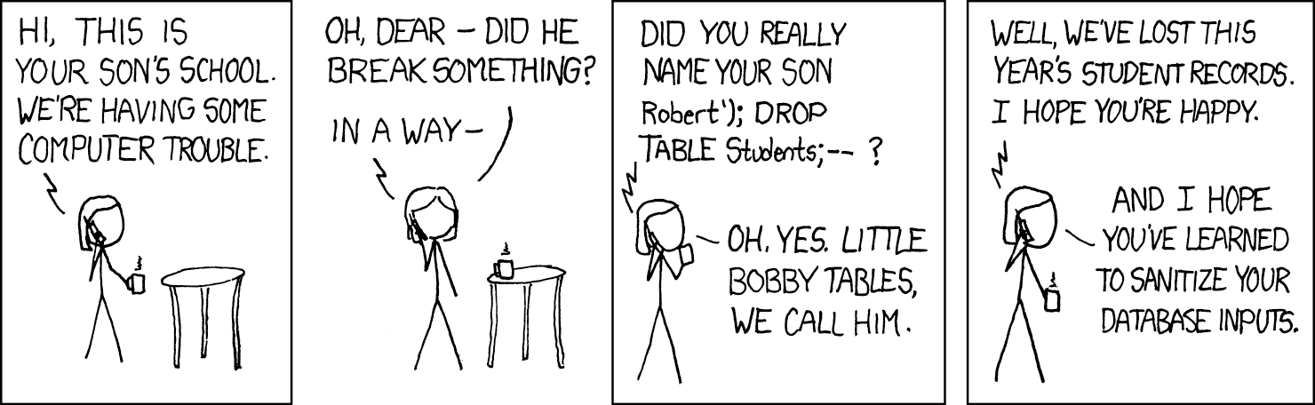
Techniques like this are required when working with forms. Hackers will actually SKIP the form and jump straight to the functions accessing the database, so anytime you are preparing to manipulate the data in your database, make sure you’ve done everything you can to ensure that, for example, what you thought was a form input asking for a name is indeed what you expect, and that you’re not executing rogue code instead.
Add recipes data
Repeat the techniques used to add the supplies data with the recipes data.
- when running as main, write a “with” statement that opens the “recipes.csv”
- write an
add_recipe()function:- where the attributes in the INSERT match the attributes set up in the
recipedata table EXCEPT for the id because that is “auto incremented” and already set for us, - and the number of
%splaceholders match the number of attributes mentioned
- where the attributes in the INSERT match the attributes set up in the
(Re-)set up the database
Run database.py to add the data to the database:
- Make sure you are connected to IU’s VPN if you are not on campus (Ivanti)
- Activate the virtual environment inside your lecture repository
- Run the database module
source venv/bin/activate
python3 -m flaskapp.database
In a terminal, log into MariaDB to check that the data is there:
SELECT supply_name FROM supplies;
SELECT recipe_name FROM recipes;
You can also do a SELECT * FROM <table>; too if you want to see all the data.
Follow Along with the Instructor
Practice with the instructor. Not an exact replacement for the written directions. Read the text below this first before proceeding.
- Refactor supplies and index routes.
Connect app.py to database.py
Connecting our application to the database is almost complete. What we need to do next is connect app.py to the database module database.py, then scan for WHERE we are working with data, and replace those interactions with calls to the database instead.
At the top of app.py lets add an import for the database module. (I chose to import with a nickname to make using the module a little simpler.)
from flask import Flask, render_template, url_for, redirect, request
from collections import defaultdict
import flaskapp.database as db
import csv
app = Flask(__name__)
Supplies refactor
Next, let’s work through each route, starting with the simplest dataset, the supplies list.
@app.route("/supplies")
def render_supplies():
all_supplies = get_all_supplies()
return render_template("supplies.html", all_supplies=all_supplies)
In the current version, we’re getting all the supply data by calling a function get_all_supplies that opens the supplies.csv and grabs all the data as a nested list.
Instead, let’s call a function in our database module to handle getting all the supplies:
# lives in app.py
@app.route("/supplies")
def render_supplies():
all_supplies = db.get_supplies()
return render_template("supplies.html", all_supplies=all_supplies)
- The function
get_supplies()lives indatabase.pyso we have to reference the module we imported before we can use the function. - Since the data in
all_suppliescan still be passed to the supplies template as is, that’s the only change we need to make.
We now need to write the function get_supplies() in database.py:
# lives in database.py
def get_supplies():
conn = get_connection()
with conn.cursor() as curr:
curr.execute("SELECT * FROM supplies")
supplies = curr.fetchall()
conn.commit()
conn.close()
return supplies
Once we have selected the supplies data, we return it back to where the function was called in app.py. We can also DELETE the get_all_supplies() function in app.py because we no longer need it!
Fetchall and Fetchone
Because we are expecting information to come back to us from the SELECT query, we need a way to grab that information for use in our application.
- fetchall() gets all data returned
- fetchone() gets the first row in the data selected
Home page refactor
- Update the “/” route (index) so
all_recipesis getting recipe data from the database - Write the function
get_recipes()indatabase.py(it should look similar toget_supplies)
Adjustment for index route
all_recipes = db.get_recipes()
Check our work
Make sure you’ve activated your virtual environment, start flask and take a look at your application in the web brower.
Uh oh 😬, the browser is displaying an error message. Let’s take a look:
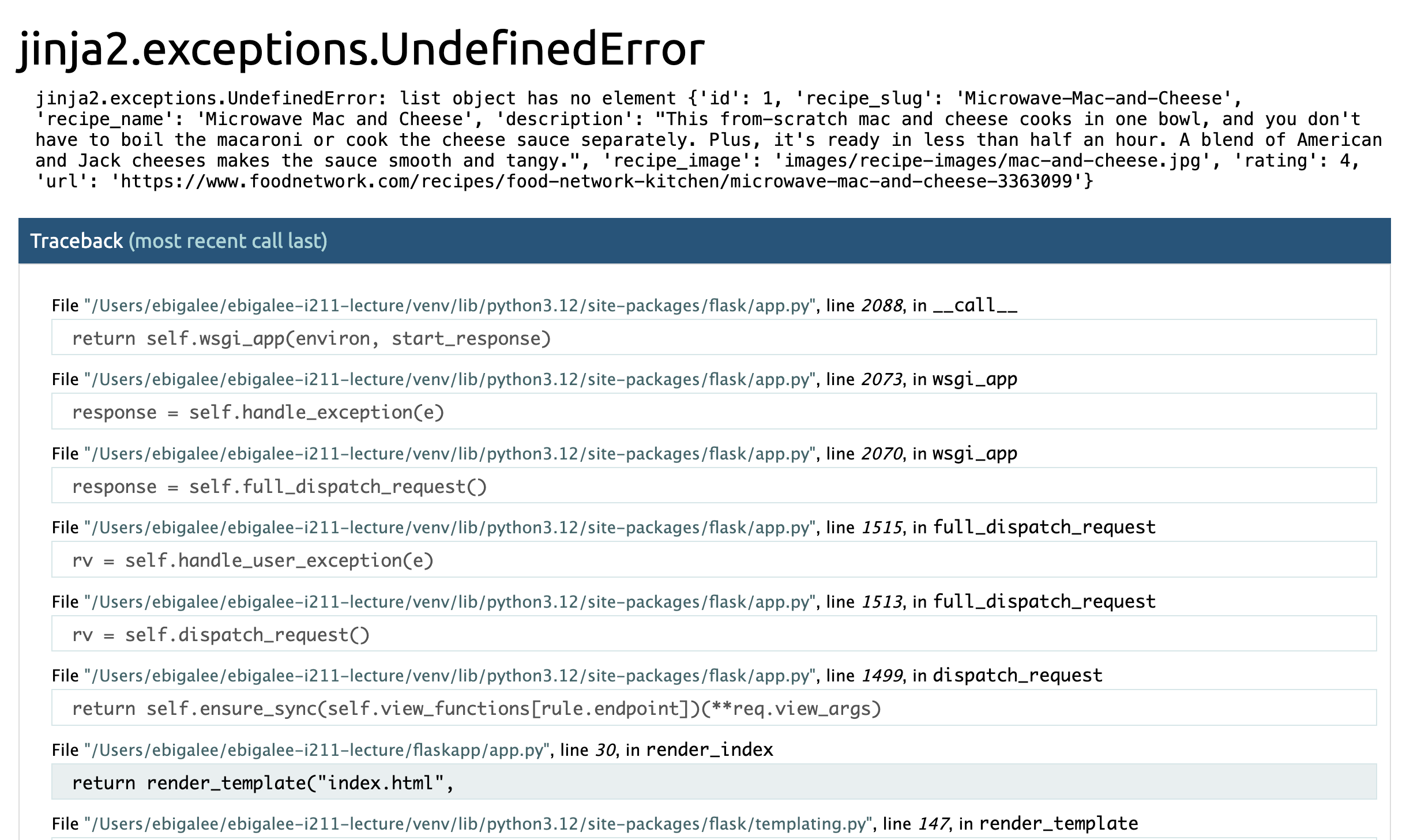
The error mentions “jinja” and sometimes errors like this will also mention “templates”. This means it’s likely an issue in one of the HTML templates.
(If that message says something about apps or python, then you know to look in `app.py’.)
Update index.html
Looks like in updating the structure of the data, we will need to make some minor adjustments to our templates as well.
Update the link to each recipe on index.html
What we want to do here is scan the error message for clues as to what went wrong. In particular the blue highlighted messages will point us in the right direction.
<a href="{{url_for('render_recipe', recipe=all_recipes[recipe]['recipe_slug'])}}">
Looks like we WERE using recipe_slug to identify each recipe, but we now have an unique id for that. We also had a DICTIONARY of dictionaries, and now we have a LIST of dictionaries.
We can see this if we jinja print all_recipes somewhere inside index.html:
{{all_recipes}}
Then we will see the data structure:
[{'id': 1, 'recipe_slug': 'Microwave-Mac-and-Cheese', 'recipe_name': 'Microwave Mac and Cheese', 'description': "This from-scratch mac and cheese...", 'recipe_image': 'images/recipe-images/mac-and-cheese.jpg', 'rating': 4, 'url': 'https://www.foodnetwork.com/recipes/food-network-kitchen/microwave-mac-and-cheese-3363099'}, {'id': 2, 'recipe_slug': '5-Ingredient-Chicken-Pesto-Soup', ...}, {}, ... ]
Which will help us update our code in index.html from:
<a href="{{url_for('render_recipe', recipe=all_recipes[recipe]['recipe_slug'])}}">
to:
<a href="{{url_for('render_recipe', recipe=recipe['recipe_slug'])}}">
The dictionary of dictionaries we has before has advantages, but as you can see, a list of dictionaries is a little shorter in this particular instance. The trick is to not make an assumption about what it should be. Print or jinja print the structure so you can see how best to access the data as you need to.
Update the link to the image for each recipe on index.html
Same issue here. We’re going from a dictionary of dictionaries to a list of dictionaries.
<img class="card-img-top" src="{{url_for('static', filename=recipe]['recipe_image'])}}" alt="{{all_recipes[recipe]['recipe_name']}}">
Once again, we need to adjust to the new data structure.
<img class="card-img-top" src="{{url_for('static', filename=recipe['recipe_image'])}}" alt="{{recipe['recipe_slug']}}">
Update the name of each recipe on index.html
Finally, we update the name of the recipe from:
<h2>{{all_recipes[recipe]['recipe_name']}}</h2>
To:
<h2>{{recipe['recipe_name']}}</h2>
The home page should be running now. If it is not, continue to debug. As you work through this adjustment, you may encounter errors in a different order, or different issue, but the process to fix them is the same. Trace the logic, trace what each variable is set to, and that usually leads to where the issue is located.
Follow Along with the Instructor
Practice with the instructor. Not an exact replacement for the written directions. Read the text below this first before proceeding.
- Refactor recipes route.
Recipe page refactor
In the route /recipes/<recipe>, we are currently getting ALL RECIPES just to be able to find the ONE RECIPE we want. Using SQL, we don’t need to get and set ALL of our database data each time we want to select a single record.
We have a better way of uniquely identifying records
To be clear about what needs to happen, let’s first update the NAME of the route to be /recipes/<recipe_id>. The data coming in from the CSV is a dictionary of dictionaries, and we are using the recipe’s slug to identify an individual recipe.
However, now we now have an unique id in the “recipes” table that we can reference instead of the slug! 🐌
@app.route("/recipes/<recipe_id>")
def render_recipe(recipe_id="None"):
...
This means we’ll need to adjust the link on index.html as well:
<a href="{{url_for('render_recipe', recipe_id=recipe['id'])}}">
The left side of the statement saying what data is being passed to app.py needs to match the top of our route @app.route("/recipes/<recipe_id>") – so we will change it to be recipe_id.
Update the recipe route and write get_recipe()
In the recipe route, call a database function called get_recipe(recipe_id) to select a single recipe matching that recipe’s ID.
@app.route("/recipes/<recipe_id>")
def render_recipe(recipe_id="None"):
one_recipe = db.get_recipe(recipe_id)
...
Now head back over to database.py to write the function get_recipe(id).
- our select is needs to be more specific - look at the INSERT examples to see how the formatting works
- the most useful fetch here is “fetchone”, which returns a single tuple. If you use “fetchall” you’ll get a tuple inside a tuple.
- don’t forget to
returnthe recipe data
Solution
def get_recipe(id):
conn = get_connection()
with conn.cursor() as curr:
curr.execute("SELECT * FROM recipes WHERE id = %s", (id))
recipe = curr.fetchone()
conn.commit()
conn.close()
return recipe
The data might be in a different format
One more issue to solve. The data coming back from fetchone is a dictionary. This might mean we need to adjust how we work with it.
{'id': 1, 'recipe_slug': 'Microwave-Mac-and-Cheese', 'recipe_name': 'Microwave Mac and Cheese', 'description': "This from-scratch mac and cheese cooks in one bowl, and you don't have to boil the macaroni or cook the cheese sauce separately. Plus, it's ready in less than half an hour. A blend of American and Jack cheeses makes the sauce smooth and tangy.", 'recipe_image': 'images/recipe-images/mac-and-cheese.jpg', 'rating': 4, 'url': 'https://www.foodnetwork.com/recipes/food-network-kitchen/microwave-mac-and-cheese-3363099'}
Notice the adjustments we made. Change them one at a time and the attempt to navigate to a recipe page in your app to see what errors are thrown. Knowing what it looks like when it’s broken can help you get comfortable with debugging.
@app.route("/recipes/<recipe_id>")
def render_recipe(recipe_id="None"):
one_recipe = db.get_recipe(recipe_id)
one_recipe['rating'] = '⭐️ ' * int(one_recipe['rating'])
return render_template('recipe.html',
one_recipe=one_recipe,
tagged_as=csv_to_tbr()['recipe_slug'],
all_tags=sorted(get_tags())
)
Our variable one_recipe was a dictionary before and is still a dictionary. This means when we click on a recipe in the home page, the recipe.html page should still work. If it does not, continue to follow this process to debug your code.
- trace each variable from where it is created in the route, through the new functions we’ve written in
database.py, and back to the route’s function, and finally on to a template. - use
print(one_recipe)in Python and{{one_recipe}}in “recipe.html”, for example, to see what a variable looks like at different points in your program. The Python print statements will log their result in the Terminal. The jinja print statements will display in your browser.
Update “Add a Recipe”
One final update based on the recipe data – the /add-recipe route.
@app.route("/add-recipe", methods=['GET', 'POST'])
def add_recipe():
if request.method == "POST":
...
all_recipes = get_all_recipes()
all_recipes[recipe_name] = new_recipe
set_all_recipes(all_recipes)
# process the form data, then go to the home page
return redirect(url_for('render_index'))
else:
# view the add recipe page
return render_template("add-recipe.html")
Most of the code here is perfectly fine. And because we take time to make new_recipe into a dictionary, all we really need to do is adjust the three lines getting and setting the data.
Try it out. Replace the following code with a call to the functions in the database module instead:
# replace me
all_recipes = get_all_recipes()
all_recipes[recipe_name] = new_recipe
set_all_recipes(all_recipes)
Solution
db.add_recipe(new_recipe)
PyMySQL and Flask II
The remaining routes in our Flask application are related to tags. Let’s begin by updating database.py. To start, we need to:
- Create a table called
taggedin the database to hold tag data - Use Python to load data from
tagged.csvinto thetaggedtable - Write a function to get all tagged data, and one to get all tags for a specific recipe
Try each of these steps on your own, checking against the solutions only after you’ve tried it.
Follow Along with the Instructor
Practice with the instructor. Not an exact replacement for the written directions. Read the text below this first before proceeding.
- Set up tagged/tags in the database.
1. Create a “tagged” data table
The first step is to update database.py to include a data table for the tagged.csv instead of a CSV.
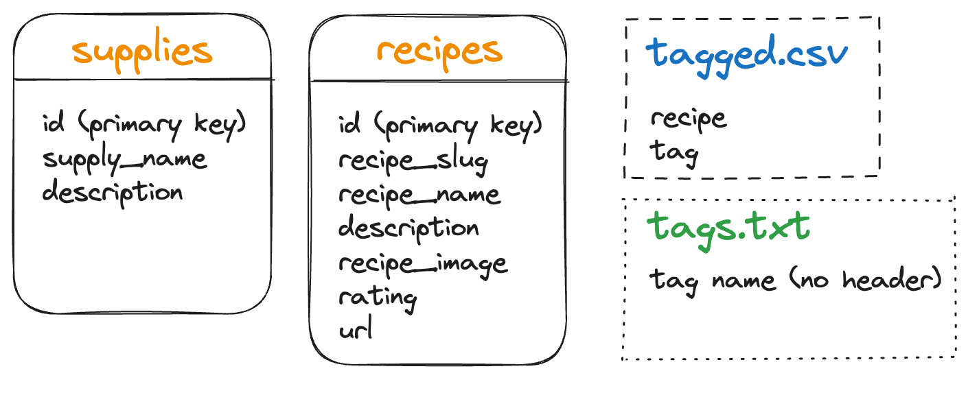
We know we need:
- integer as the primary key for the
id(our unique identifier)
Looking at tagged.csv to see what other attributes and datatypes to include we see:
- recipe (currently the recipe’s slug)
- tag
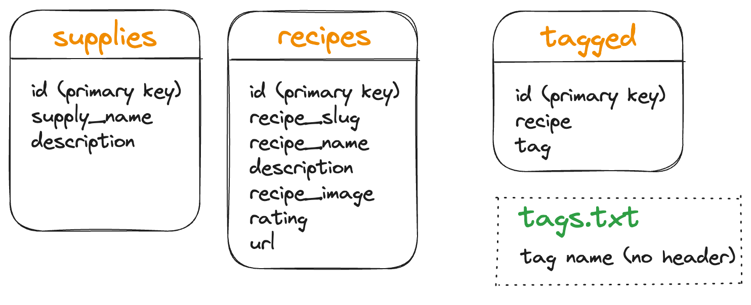
Just because the CSV was set up a certain way DOES NOT MEAN that the database should be the same. Because we now have a relational database, it makes sense to connect to the full recipe record in the recipes table – to establish a relationship.
Caveat: there are many ways to structure data and design a database. Whole courses exist to teach you just this. The choices made here are deemed most instructional for THIS course.
Connect tables using a foreign key
When we connect one table to another, that is indicated by a foreign key or the reference ID from another table.
CREATE TABLE tagged (
...,
constraint `fk_recipe_id`
foreign key (recipe_id) references recipes(id),
) engine=InnoDB;
To set recipe_id as the foreign key we set a constraint and give it a name. One convention is to call this fk_<attribute> meaning “foreign key for the specified attribute”. We then set the foreign key to be an attribute in our current data table, and list what attribute the key will reference in another table.
- One more time 😅: this says constraint “fk_recipe_id” is a foreign key called “recipe_id” and its value is an id from the “recipes” data table.
Instead of a column of recipe names in slug form, we now have a column with a unique id pointing to the record for a recipe.
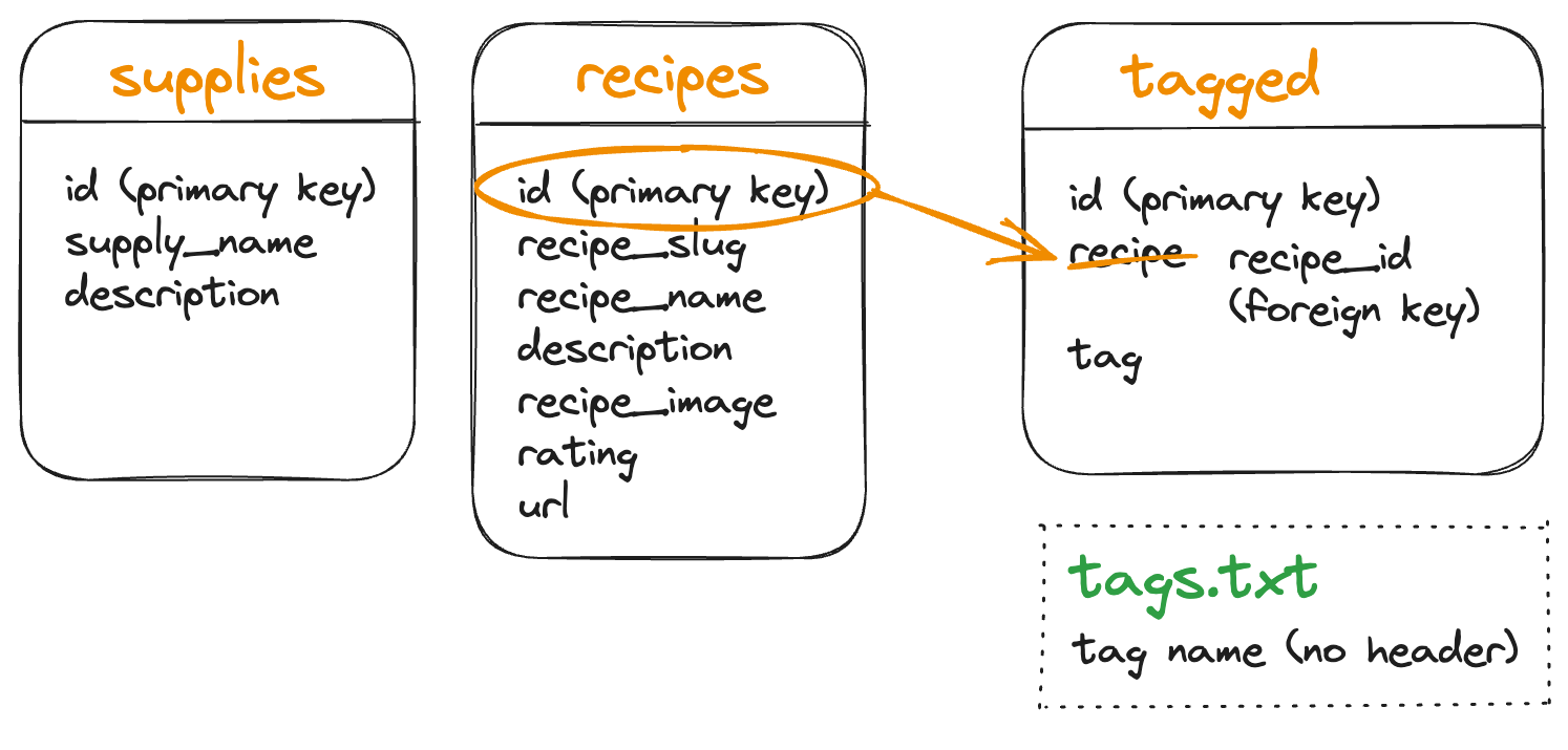
We can now eliminate the “tags.txt” file
We also have a text file listing all of the possible tags. Again, because this information will be stored in the database, it makes the most sense to simply pull in all tags in tagged to create a list of tags.
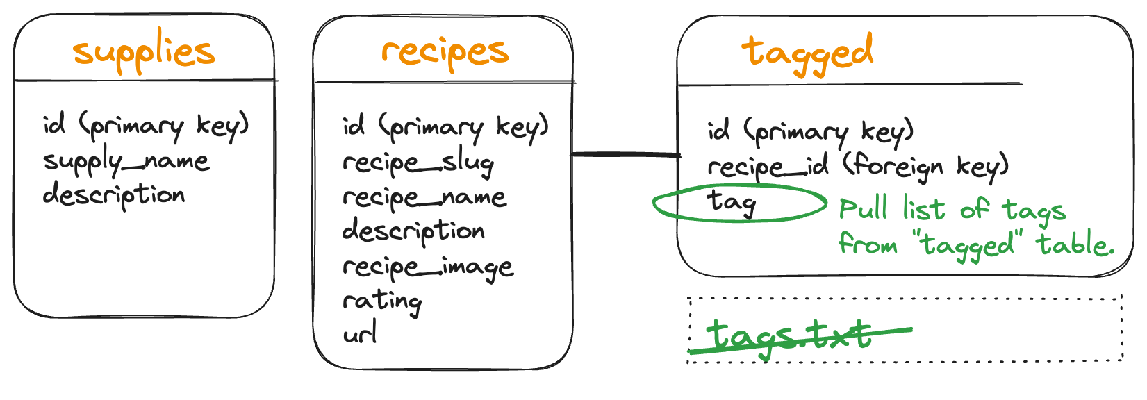
(Depending on future plans for the tags, a table could be created just to hold those possibly tag names. We don’t plan to go further with this app, so this choice finishes our database design and eliminates the need for CSVs and TXT files beyond the inital loading of some data.)
Possible Solution for Adding the Tagged Table
def initialize_db():
...
_tagged = """
create table tagged (
id int auto_increment primary key,
recipe_id int,
tag varchar(25),
constraint `fk_recipe_id`
foreign key (recipe_id) references recipes(id)
) engine=InnoDB
"""
Note: We MUST DROP THE TAGGED TABLE FIRST. This is because the foreign key is linked to the recipes table. That dependency will keep the “drop table” command from executing, so easiest is just to drop “tagged” first.
Possible Solution for Adding the Tagged Table Continued...
def initialize_db():
...
with conn.cursor() as curr:
curr.execute("drop table if exists tagged")
curr.execute("drop table if exists supplies")
curr.execute("drop table if exists recipes")
curr.execute(_supplies)
curr.execute(_recipes)
curr.execute(_tagged)
conn.commit()
conn.close()
2. Load CSV data into the “tagged” table
We made changes to how the data is structured, so we’ll need to adjust our initial data to match if we still want to bring in the “tagged” data from the CSV.
Update “tagged.csv”
Replace the current text in tagged.csv with the following. Instead of a “recipe” holding a slug, we now have a “recipe_id” holding the ID for the recipe that appears in the “recipes” data table.
recipe_id,tag
1,vegetarian
1,cheese
1,breakfast
4,pasta
4,vegetarian
5,vegetarian
6,vegetarian
6,drinks
6,breakfast
3,rice
10,rice
Once the tagged.csv files is updated, let’s continue to update database.py.
Pull the data from “tagged.csv” into our database
Use Python and PyMySQL to pull the data out of tagged.csv and insert it into the tagged data table. This includes opening the CSV and looping through the available records…
Possible Solution for Pulling in Data from Tagged CSV
if __name__ == "__main__":
initialize_db()
...
with open("tagged.csv") as csvf:
for tagged in csv.DictReader(csvf):
add_tagged(tagged)
…as well as writing a function to help you add each row of data to the data table.
Possible Solution for Adding Data to Tagged Table
def add_tagged(tagged: dict[str, str]) -> None:
conn = get_connection()
with conn.cursor() as curr:
curr.execute(
"insert into tagged (recipe_id, tag) values (%s, %s)",
(
tagged["recipe_id"],
tagged["tag"],
),
)
conn.commit()
conn.close()
The INSERT is referencing the attributes in the new CSV file.
Re-initialize our database
Re-run the database.py file and re-initalize the tables, initial data in the tables, and set up the functions we’ll be using inside our app. See PyMySQL and Flask 1 for details.
Remember, this will delete any data we had updated in the app, so we won’t want to initialize everything again once our app is in production. Designing, planning and implementing a database is something that should be done with care. Once we begin to use the database, it becomes much harder to make adjustments. 😓 For this lecture repo, we’re just starting over each time we make a change.
Follow Along with the Instructor
Practice with the instructor. Not an exact replacement for the written directions. Read the text below this first before proceeding.
- Set up helpful function to access tags in the database
- Refactored the index route to handle tags
3. Write a function to get all data from the “tagged” table
To best access this tagged data, we should to be able to:
- grab the contents of the entire “tagged” data table
- make a specific selection to get the tags applied to an individual recipe
- select all of the tags in use
We can take this one step further and translate this need into pseudo code.
Update database.py by writing the following functions:
get_all_tagged()to select all of the records from thetaggedtableget_tags(recipe_id)to select the tags applied to the recipe indicated by the idget_all_tags()to select all of the tags present in the tagged table
Get all tagged recipes:
Possible Solution for a Function to "Get All Tagged" Recipes
def get_all_tagged():
conn = get_connection()
with conn.cursor() as curr:
curr.execute("SELECT * FROM tagged")
all_tagged = curr.fetchall()
conn.commit()
conn.close()
return all_tagged
Get all tags for a single recipe:
Possible Solution for a Function to "Get Tags" for a Recipe
def get_tags(recipe_id):
conn = get_connection()
with conn.cursor() as curr:
curr.execute("SELECT * FROM tagged WHERE recipe_id = %s", (recipe_id))
tags = curr.fetchall()
conn.commit()
conn.close()
return tags
Get all tags in use:
For get_all_tags() we have options.
We can say SELECT tag FROM tagged; and get all of the tags in the data table, however, this includes duplicate tags, which we have quite a few of.
- Option 1: Using Python in
app.pywe could then filter those tags into a list of unique tags. - Option 2: We can use the SQL keyword “DISTINCT” and that will limit our selection.
SELECT DISTINCT tags FROM tagged;
You may implement whichever way makes the most sense to you.
Possible Solution for a Function to "Get All Tags" Currently Used
def get_all_tags():
conn = get_connection()
with conn.cursor() as curr:
curr.execute("SELECT DISTINCT tag FROM tagged")
all_tags = curr.fetchall()
conn.commit()
conn.close()
return all_tags
Updating the tagging system in our application
Now we switch over to app.py to make use of all our hard work on the database and in PyMySQL.
In each of these routes, do not copy and paste this code in. Instead find where there are changes between your current code and the code we provide below, then adjust line by line as needed.
We really want you to see where changes need to be made and (eventually) how much simpler the code will now read without the mess caused by trying to use a CSV as our only data source.
Update / route
The data coming back from db.get_all_tagged() is a list of dictionaries:
[{'id': 1, 'recipe_id': 1, 'tag': 'vegetarian'}, {'id': 2, 'recipe_id': 1, 'tag': 'cheese'}, {'id': 3, 'recipe_id': 1, 'tag': 'breakfast'}, {'id': 4, 'recipe_id': 4, 'tag': 'pasta'}, {'id': 5, 'recipe_id': 4, 'tag': 'vegetarian'}, {'id': 6, 'recipe_id': 5, 'tag': 'vegetarian'}, {'id': 7, 'recipe_id': 6, 'tag': 'vegetarian'}, {'id': 8, 'recipe_id': 6, 'tag': 'drinks'}, {'id': 9, 'recipe_id': 6, 'tag': 'breakfast'}, {'id': 10, 'recipe_id': 3, 'tag': 'rice'}, {'id': 11, 'recipe_id': 10, 'tag': 'rice'}]
But it’s more helpful to us if it is organized as a dictionary where the key is the recipe_id and the value is a list of all tags assigned to that recipe:
{1: ['cheese', 'breakfast'], 4: ['vegetarian'], 5: [], 6: ['drinks', 'breakfast'], 3: [], 10: []}
To do this, it’s helpful to write a function:
def make_tags_by_recipe(all_tagged: list[dict]) -> dict[list]:
tags_by_recipe = {}
for tagged in all_tagged:
if tagged['recipe_id'] in tags_by_recipe.keys():
tags_by_recipe[tagged['recipe_id']].append(tagged['tag'])
else:
tags_by_recipe[tagged['recipe_id']] = []
return tags_by_recipe
This allows us to simplify the code in our route:
@app.route("/")
def render_index():
all_recipes = db.get_recipes()
all_tagged = db.get_all_tagged()
tags_by_recipe = make_tags_by_recipe(all_tagged)
return render_template("index.html",
all_recipes=all_recipes,
tags_by_recipe=tags_by_recipe
)
Code that changed in the “index.html” template:
...
{% for tag in tags_by_recipe[recipe['id']] %}
<span class="badge rounded-pill text-bg-success">{{ tag }}</span>
{% endfor %}
Follow Along with the Instructor
Practice with the instructor. Not an exact replacement for the written directions. Read the text below this first before proceeding.
- Update the recipes/recipe_id and add tag routes.
- Complete the lecture application, including deploying.
Update /recipes/<recipe_id> route
Two updates to the data here, tagged_as to show which tags the recipe has, and all_tags which populates the dropdown in the form to add a new tag.
tagged_as
For tagged_as, we want to use db.get_tags(recipe_id) to get all the tags the current recipe has applied. The format in this case is fine, and we can use jinja to unpack it in “recipe.html”:
[{'id': 1, 'recipe_id': 1, 'tag': 'vegetarian'}, {'id': 2, 'recipe_id': 1, 'tag': 'cheese'}, {'id': 3, 'recipe_id': 1, 'tag': 'breakfast'}]
Code that changes in “recipe.html” template:
{% for tag in tagged_as %}
<span class="badge rounded-pill text-bg-success">{{tag['tag']}}</span>
{% endfor %}
all_tags
The dropdown on “recipe.html” needs a simple list of tags, yet we see that when we call db.get_all_tags(), it’s currently a list of dictionaries.
[{'tag': 'vegetarian'}, {'tag': 'cheese'}, {'tag': 'breakfast'}, {'tag': 'pasta'}, {'tag': 'drinks'}, {'tag': 'rice'}]
Putting just the tag names into a list will do the trick.
def make_clean_tags(all_tags: list[dict]) -> list:
return [tag['tag'] for tag in all_tags]
['breakfast', 'cheese', 'drinks', 'pasta', 'rice', 'vegetarian']
Using a helper function makes our route’s function a little simpler too. If you’re not familiar with list comprehensions, the code in make_clean_tags is the same as saying:
clean_tags = []
for tag in all_tags:
clean_tags.append(tag['tag'])
Sorting those tags in place gives us a nice way to send the data on to the template where it’s displayed in a dropdown menu.
Updated recipe route
@app.route("/recipes/<recipe_id>")
def render_recipe(recipe_id="None"):
one_recipe = db.get_recipe(recipe_id)
one_recipe['rating'] = '⭐️ ' * int(one_recipe['rating'])
all_tags = make_clean_tags(db.get_all_tags())
return render_template('recipe.html',
one_recipe=one_recipe,
tagged_as=db.get_tags(recipe_id),
all_tags=sorted(all_tags)
)
Update /api/tags/<recipe_id>/add route
The code here changes quite a bit, and is for the most part simpler because we now have specific functions in database.py handling the needed selections.
@app.route("/api/tags/<recipe_id>/add", methods=["POST"])
def add_tag_to_recipe(recipe_id: str):
added_tag = request.form["tag_name"]
if not added_tag:
return "Bad request, missing tag name", 400
if not recipe_id:
return "Bad request, missing recipe", 400
if not db.get_recipe(recipe_id):
return "Bad request, unknown recipe", 400
# need way to keep out duplicates
db.add_tagged(
{
"recipe_id": recipe_id,
"tag": added_tag
}
)
return redirect(url_for("render_recipe", recipe_id=recipe_id))
We’re also going to adjust the forms in “recipe.html” to handle the adjustment to the add_tag_to_recipe route, and the recipe’s id being passed along.
<form action="{{ url_for('add_tag_to_recipe', recipe_id=one_recipe['id']) }}" method="POST" class="row g-3 my-4">
Validating the tags
Right now, if we want to add a tag “fancy” and we want to add it again, there is nothing stopping us! 🎩 Additionally, there is no check on whether the tag the user came up with even SHOULD be added.
The first part - duplicates - is a straightforward fix:
if the tag is NOT present in the "tagged" table for THIS recipe:
# add tag to tagged data table
else:
# send along an error message to appear in the template
See if you can write this condition.
That second part is a harder problem that we’d need to think about. Do tags get reviewed and approved by a person? Is there a set of guidelines for what will be accepted? Or perhaps it doesn’t matter; it’s any tag goes. This is a case of us not thinking through how the site will be used and how that impacts the data needs.
We’re here at the end of our development for the recipe site though, so those are all future problems 🔮 to consider more strongly in your next application.
We don’t need the helper function anymore?
Now that we’ve used that “make_clean_tags” helper function twice, and we’re at the end of our app’s spec, we might now know that we just always need that list-of-dictionaries format. Should we determine that is what we want everytime that data is pulled, we could delete the make_clean_tags helper function and all references to it in app.py and instead add the reorganization step to the get_all_tags function in database.py:
def get_all_tags():
...
# clean up the tags to be a list
return [tag['tag'] for tag in all_tags]
This is totally optional to do today.
Functions we can now delete in app.py
In app.py we can delete the functions we used to work with CSVs!!! 😮
- import csv
- get_all_recipes()
- tbr(all_tagged)
- get_all_supplies()
- get_tags()
- csv_to_tbr()
- set_all_recipes(all_recipes)
- tbr_to_csv(tbr: dict[str, set[str]])
- register_new_tag(tag_name: str)
Your app.py should now look dramatically cleaner, clearer and more manageable.
Time to Wash the Dishes? 🍽️
We’re at the end of our build for 🍳 Make This Now!. You created a modern, fullstack web application! We’ve spent a lot of time “cooking. Are you hungry 🤤?
(In terms of the amount of work we put in for this small site with limited data, you might be questioning whether it even qualifies for a fullstack application treatment! 🤨)
A site with A LOT OF DATA or A LOT OF PAGES is really going to benefit from all this structure (and we did need to start somewhere). So if we need a site to be able to “scale” this is what we mean – a site with a structure that can handle 5 pages, but also scale to 5000.
Course Wrapup
In completing this course, you now have a much better idea of what modern software development looks like, how a full-stack web application is built, and (we hope!) feel a sense of accomplishment at what you’ve built.
Take a moment to be proud and celebrate! 🥳
Before and After
This is (probably) what your resume looked like at the start of this course:
- Technical Skills: Python, HTML
We covered so much that simply having a “Technical Skills” section is no longer precise. Your technical skills span the database to the front end and everything in between:
- Development Tools: git, GitHub, Visual Studio Code (VS Code)
- Platforms: Linux/Unix-like operating systems, Ubuntu, Windows Subsystem for Linux (WSL)
- Backend: Python, Flask framework
- Frontend: HTML, Bootstrap, Jinja
- Databases: MariaDB, SQL, pymysql
Cleanup?
Once you have a grade for this course, it should be safe to clean up the contents of your cgi-pub directory on Silo. Directories probably have names similar to the following:
first-website- described in the Networks and Servers chapterps-01USERNAME-ps-02USERNAME-ps-06i211-projecti211-lecture
What’s next?
The material we covered has many names: full-stack development, information systems, information architecture, or information infrastructure. What these phrases have in common is that they deal with computing across many layers of abstraction.
- People
- Application software
- High-level software
- Low-level software
- Operating systems
- Hardware
- Electricity
Here, we borrow layer from ideas in complex systems. A layer or layer of abstraction is a way to think about a system: and each layer works by “talking” to the layer beneath it. How do people interact with computers? — using application software. How does hardware work? — using electricity. What is the operating system? — a program that manages the underlying hardware.
The final system we built was application software: it was intended to help a user accomplish a task—such as bookmarking recipes or tagging them for easy searching. In order to build that application software, we had to write high-level software in Python to manage data and application state. That software we wrote was built on top of lower levels of abstraction: Python, Flask, Bootstrap, and many re-usable components. In order to make this system work: we needed to know enough about operating systems to store our data and run our code.
In other words, we focused our time on three layers of what is really a 7-layer information system:
- People
+ Application software
+ High-level software
- Low-level software
+ Operating systems
- Hardware
- Electricity
No matter where you go in your informatics career, you will be working at the intersection of a few of these layers.
- (I300 - HCI) Human Computer Interaction & Design: How do people interact with application software? How can application software be improved to better meet their needs?
- (I311 - App Development) Android App Development: How do we build application software for Android?
- (I360 - Web Design) Static Website Design and Usability: How do we design user-friendly professional web interfaces?
- (I365 - JavaScript) Frontend Programming Language: How do we create interactive web interfaces?
- (I399 - Data Analysis) Data Science: How do people make decisions? How can application software support their decisions?
- (I399 - Cloud) Cloud Computing: How do we virtualize everything between the application and the hardware?
Work Session v1.0.0
Read the directions for the Project
- View the assignment in Canvas
- Canvas > Modules > Week 5 > What to Do in Week 5, or
- Canvas > Modules > Week 6 > What to Do in Week 6
Sketch the interactions
This time when we sketch the user interactions, we’ll still keep the same format in our sketch where we indicate pseudo code and what data is being used at each step. We’ll still be gathering form data from the user. But CSVs are now only a way for us to load initial data, and our data will come from interactions with a database instead.
In our sketch today, let’s focus on the flowers route, which you should already have set up. The route will now need to be updated for use with a database – feel free to reference your previous sketches.
Divide a piece of paper into three sections.
- Label the first section index.html
- Label the second section app.py
- Label the third section flowers.html
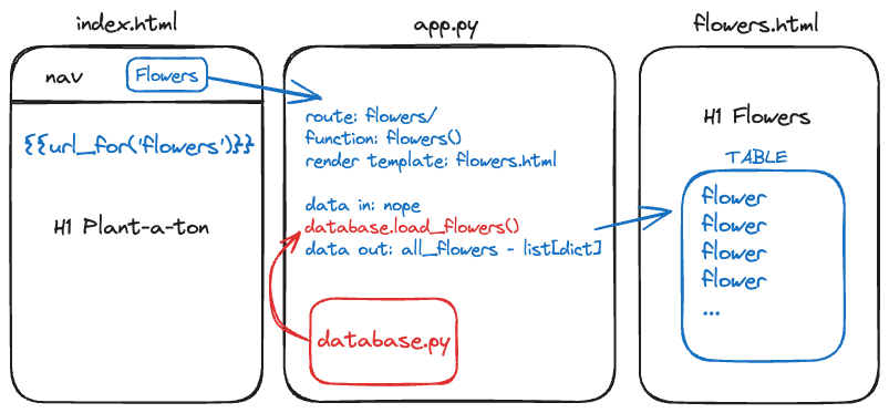
In the first section, the user clicks on “Flowers” in the navigation.
- Write the link (using Jinja and url_for())
Draw an arrow to the middle section.
In the second section, indicate:
- Route:
/flowers/ - Function definition:
flowers() - Template to render:
flowers.html - Is there any data coming in from the first section? no
- Is there any that needs to be processed or gathered? yes, “flowers” database table
- Is there any data to send on to the HTML template? yes, “all_flowers”
Don’t worry about writing the code here. Just write down the important bits.
Draw an arrow to the third section. Indicate any data that has been passed to the page, and note what the page is for (e.g. all_flowers, a list of dictionaries)
Repeat this process for the rest of the routes we have asked you to create. Reference your interaction sketches as you code.
Begin coding
Begin coding, keeping in mind the entire user interaction from a click on a link, to the route in app.py, to the resulting rendered HTML template.
Advice from Past Students
We asked the i211 students from the 6-week summer 2024 session if they had any advice for future students. Be aware some advice is tailored specifically to the summer semester, which is a particularly intense version of this course.
What would have helped you to know going in?
Advice I would give to a student taking this course next summer:
“Most Important Thing - Spend the time and practice early in the week. Spend at least 1-2 hours a day M-W practicing, watching the videos (which are very helpful). Then spend Thursday and Friday doing the Practice Sets, assignments. If you spend time practicing with the material early in the week it will give you an opportunity to go to office hours and you can ask a ton of questions, so then when you complete the projects and assignments on Thursday and Friday, you can mitigate the number of questions you may have.”
“What helped me a lot in this course was taking the time to sit down and really understand the material. It’s important to actively learn and grasp the concepts. Also, try experimenting with the code and finding new ways to solve problems. This hands-on practice can strengthen your understanding and make learning more fun.”
“stay very on top of your work in case you need help”
“My advice would be to not take this class with other classes, and be mindful of your work schedule if you have a job as well. I took this class with 1308 and a summer job, which was very hard and I basically had to say goodbye to my summer life. Students should know how much work actually goes into this class. I think this class was set up perfectly, so I can’t think of anything that should be changed. The videos were great, and even if you do run into a problem there is always people to help. I don’t think I could have changed anything because I did a LOT of studying and homework everyday.”
“This is a time-consuming class. Don’t expect this to be a breeze and make sure you dedicate a lot of time to really learn the material. I think more helper videos could be a great addition to the material.”
“My advice to a student next summer would be to do each day as it comes. Don’t stack homework days. Be ready to commit an additional hour beyond the material to make sure you actually understand what it is in a more significant degree.”
“The one piece of advice would be to not procrastinate, especially if you believe the course is easy after week 1. It is easy to fall behind and lose the flow of doing the assignments and lectures. If you follow the format of how the work is supposed to be completed, this course is not difficult to do and does not eat time outside of the week by a lot.”
“My advice is to work on the content at least for a couple hours each day. Waiting until last minute on an assignment’s due date will make you stressed out and most likely not be able to turn it in, in time. Overall, this course worked very well for me and I loved learning from this team. However, I found the last module the hardest to learn, so study and go through each step!”
Epilogue
Acknowledgements
A huge thanks to students and colleagues who caught typos, bugs, or submitted reports:
- Abe Stone (#7)
- Aidan Jameson Neel (#8)
- Isaiah Solomon Jones (#8, #15)
- Julia Macias (#9)
- Molly J. Carter (#12)
- Dalton K. Hicks (#13)
- Pengfei Zhang (#10)
- Molly J. Carter (#12)
- Vanessa Cecillia (#23)
- Kevin J. Farrell (#24)
- Dane Marshall Smith (#25)
- Sydney S. Johnson (#26, #31)
- Hudson Rose Custer (#27)
- Gavin G. Gilb (#28)
- Rowan Kylie Palmer (#29)
- Drew Henry Duncan (#33)
- Seneca Simon (#35)
- Erik G. Walker (#62, #63)
And a huge thanks to the students who helped run i211 labs and work with students:
- Ahna Abraham
- Mary Bekova
- Shibani Dcosta
- Shreeja Deshpande
- Andrew Edinger
- Johnathan Engleking
- Akhila Eshapula
- Chirayu Gupta
- Dylan Jacoby
- Satwick Kulkarni
- Steve Mendis
- Honey Patel
- Gavin Simpson
- Eli Taylor
- Namith Telkar
- Susheel Thimlapur
Many points were inspired by a need for introductory material on topics like git, shells, and text editing:
- Some of the topics were inspired by the topics in “Missing Semester,” by Anish Athalye, Jon Gjengset, and Jose Javier Gonzalez Ortiz.
- Alexander’s thoughts on teaching
gitwere heavily inspired by a 2018 blog post by Rachel M. Carmena called How to teach Git and the related material.
Teaching with this book
Alexander started writing this book during summer 2023, while assisting with course material for I210 and I211. Erika began editing and writing for the book during the summer of 2024 in preparation for teaching I211 online and asynchronously.
The book is a work in progress - if you find an error or have a suggestion, please reach out to your current I211 instructor.