Structured Data II: SQL
Are you seeing the limitations of using text files and CSV files yet? They are frequently the simplest and fastest way to get a minimum viable product in front of users: just store and load data from files on the operating system.
But perhaps you’ve also been bitten by one or more of their limitations.
Perhaps you made a mistake when writing to a file. Perhaps you started with a text file that contained data:
$ cat data.txt
1
2
3
… and you wanted to update this file by putting the number 4 after the 3:
>>> with open("data.txt", "w") as fh:
...     fh.write("1\n2\n3" + 4 + "\n")
...
Traceback (most recent call last):
  File "<stdin>", line 2, in <module>
TypeError: can only concatenate str (not "int") to str
Oops. We made an honest mistake while updating the file. But our honest mistake erased data.txt:
$ cat data.txt
$
Perhaps you were annoyed that everything was a string. Even if there were a column similar to “age” where everything looked like a numeric value:
$ cat turtles.csv
"species","length","age"
"Spotted","5.0 5.0",92
"Spotted","5.1 4.9 5.0",30
… there is nothing in the CSV specification to guarantee this observation, so the default behavior made by Python’s csv standard library (and many similar implementations) is to represent every piece of data as a string:
import csv
from pprint import pprint

with open("turtles.csv") as csvf:
    pprint(list(csv.DictReader(csvf)))
$ python3 stringly_typed.py
[{'age': '92', 'length': '5.0 5.0', 'species': 'Spotted'},
 {'age': '30', 'length': '5.1 4.9 5.0', 'species': 'Spotted'}]
Perhaps you noticed we had to save and load the whole file every time. When we wanted to modify a single row in a CSV file, we showed that we had to load the entire thing, perhaps with Python’s csv.DictReader, update it, and write it back out with csv.DictWriter:
import csv

# Read the *entire* dataset into Python
with open("turtles.csv") as csvf:
    data = list(csv.DictReader(csvf))

# Write the *entire* list-of-dictionaries back to a file
with open("turtles.csv", "w") as csvf:
    writer = csv.DictWriter(csvf, fieldnames=["age", "length", "species"])
    writer.writeheader()
    writer.writerows(data)
… for tiny datasets this isn’t necessarily a problem. But what if our file was 10× bigger? or 100× bigger? Our application would become slower proportional to how big our files were. But what if our data was 100 gigabytes and did not fit in our computer’s main memory?
Data storage guarantees, data types, and partitioning data into logical groups are some of the guarantees that a database provides. A database is a program providing a standardized way to store and query data. Many types of databases exist, each specialized to handle the data storage and querying needs of particular groups of people (a few off the top of Alexander’s head: NoSQL, graph databases, vector stores, search engines, blob storage, key-value stores).
In other words—for any problem that you can imagine, there is an implicit data storage and data management problem. We will avoid most of these choices and complexities (they are topics for another course). Instead we will focus on three types of data modeling approaches. We’ve already encountered two of them:
- Hierarchical data or tree-structured data, which is how we represented file system and the object references used in many programming languages.
- Graph data, which is how we described the structure of the Internet and other means of human communication.
There is one final idea that we want to cover as we draw near the conclusion of this course. When Edgar F. Codd proposed the relational model in 1970,1 he invented it specifically as a way to counter problems that arise when storing data using the previous two approaches.
- Relational data, where data are represented as discrete sets of items, and relations between items.
This idea: storing databases of tuples and relations has proved invaluable for the last fifty years. The relational model, relational databases based on the relational model, and the relational database management systems (RDBMS) comprised of the former.
Today we:
- introduce the relational model,
- its implementation in the MariaDB RDBMS, and
- its creation and querying with structured query language (SQL).
Follow Along with the Instructor
Not an exacty replacement for the book, but let’s highlight some major points together and introduce the relational model.
From tabular to relational data
Edgar F. Codd proposed the relational model in 1970 while working as a programmer at IBM.1 The key ideas were derived from set theory, tuples, and relations defined on related sets of tuples.
Remember how we began the CSV chapter with an example where we were buying groceries for Alice and Bob?
| name | aisle | for |
|---|---|---|
| milk | 24 | Bob |
| cheese | 23 | Bob |
| eggs | 19 | Alice |
| chicken noodle soup | 6 | Alice |
| chicken noodle soup | 6 | Bob |
Now imagine that we also had to represent other information about the people that we were shopping for. Alice and Bob probably have phone numbers and addresses:
('Alice', '123-1122', '123 Street Ave.')
('Bob', '113-7812', '124 Avenue St.')
How would we put data about their phone numbers and addresses into the existing table? We could add new columns for phone numbers and addresses, but now we’ve effectively duplicated our data. Every time we see the name “Alice” or “Bob” have to copy their phone number and address into that row:
| name | aisle | for | phone | address |
|---|---|---|---|---|
| milk | 24 | Bob | 113-… | 124 Av… |
| cheese | 23 | Bob | 113-… | 124 Av… |
| eggs | 19 | Alice | 123-… | 123 St… |
| chicken noodle soup | 6 | Alice | 123-… | 123 St… |
| chicken noodle soup | 6 | Bob | 113-… | 124 Av… |
This exacerbates an earlier problem: we have multiple “chicken noodle soup” rows, and multiple “people” rows. If we had to update this data at a later point in time, we’d have to be mindful of all the places we’ve copy-and-pasted the data and make sure we change them in every single location.
We’ll call this a data normalization problem in a bit. The relational model would propose that instead of the flat tabular data representation, we could instead model the three concepts underlying our problem:
- people: with names, phone numbers, and addresses
- groceries: which are located on a particular aisle
- orders: which people want which groceries?
Rather than trying to force these facts into one giant table, we could instead split them into three smaller tables that each focus on a particular part of our data:
| person | phone | address |
|---|---|---|
| Bob | 113-… | 124 Av… |
| Alice | 123-… | 123 St… |
| name | aisle |
|---|---|
| milk | 24 |
| cheese | 23 |
| eggs | 19 |
| chicken noodle soup | 6 |
| name | for |
|---|---|
| milk | Bob |
| cheese | Bob |
| eggs | Alice |
| chicken noodle soup | Alice |
| chicken noodle soup | Bob |
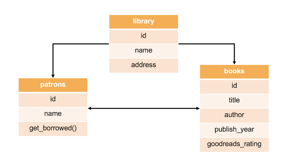
Each table represents a relation. Each column represents an attribute of that relation, and the total number of columns in a table corresponds to the relation’s arity (binary, ternary, etc.). These concepts provide an abstraction: a higher-level representation of how data are stored and eventually queried. One could look at a high-level picture of the data, such as is shown in an entity-relationship diagram,2 without needing to see every tuple. We decomposed the giant table into a series of relations between attributes: “people place orders”, “an order contains groceries”:
erDiagram
    PERSON {
        string name
        string phone
        string address
    }
    GROCERY {
        string name
        int aisle
    }
    GROCERY }o--o{ ORDER : containing
    PERSON }o--o{ ORDER : places
This decomposition is closely related to what Codd and others call data normalization. The precise nature of normalization requires several other concepts. Briefly: what would happen if there were two people who were named Alice?
| person | phone | address |
|---|---|---|
| Bob | 113-… | 124 Av… |
| Alice | 123-… | 123 St… |
| Alice | 112-… | 125 St… |
We previously assumed that every name was unique. Therefore when we kept track of each person’s order we put in their name and the item they wanted. But if there were two people named “Alice”, we can no longer look at this entry and know who an order belongs to:
| name | for |
|---|---|
| … | … |
| eggs | Alice |
| chicken noodle soup | Alice |
| … | … |
Codd introduced this as a problem of cross-referencing data between two relations, but also showed there was a “a user-oriented means” of fixing this: unique identifiers called keys which could reference individual pieces of data. Keys came in two varieties: primary keys that uniquely identify each piece of data, and foreign keys which refer to or reference keys inside other relations.
In our person table, we can introduce an id attribute. Identifier attributes that uniquely identify every piece of data rarely occur naturally. Here we will invent an identifier, a primary key integer that starts at 1 and increments every time we need a new person:
| id | person | phone | address |
|---|---|---|---|
| 1 | Bob | 113-… | 124 Av… |
| 2 | Alice | 123-… | 123 St… |
| 3 | Alice | 112-… | 125 St… |
Now we can replace everywhere that previously referred to the first Alice with her foreign key: 2 referencing the id attribute in our other table:
| name | for |
|---|---|
| … | … |
| eggs | 2 |
| chicken noodle soup | 2 |
| … | … |
Now we’re ready for an imperfect but nevertheless good-enough definition of normalization: a fully normalized3 data set is one without redundancy, where every row which can be uniquely identified is uniquely identified, and when we need to cross reference data we do so through primary and foreign keys. Normalized data is often useful: if we need to change something then we only need to change it in one location, as opposed to that giant CSV we started with where changing a person’s address would require updating multiple rows of data.
So far our discussion is high-level and theoretical. In reality: we have to deal with questions like: Where does data come from? How do we define a relation? How do we add or remove data over time? We’re ready to interact with an implementation of the theoretical model: in the MariaDB database.
MariaDB
There are many variants of relational databases to choose from, just like there are many flavors of Linux available. If you’ve heard of any of them, you’ve likely heard of Oracle, MySQL, or Microsoft SQL Server. In Informatics, we use MariaDB, which is a fully open-source variant of MySQL.
Log into MariaDB. Begin by logging into the SICE server “SILO” using your IU credentials:
ssh USERNAME@silo.luddy.indiana.edu
You should see a starred banner. From the command line when logged into Silo, we can additionally access the database accounts set up for us:
mysql -h HOST -u USERNAME --password=PASSWORD -D DATABASE
HOST, USERNAME and DATABASE are replaced by your own credentials.
SICE has set an account up for you. These credentials are available in Canvas - see the current week’s page.
$ mysql -h HOST -u USERNAME --password=PASSWORD -D DATABASE
Welcome to the MariaDB monitor.  Commands end with ; or \g.
Your MariaDB connection id is 171566
Server version: 10.6.18-MariaDB-0ubuntu0.22.04.1 Ubuntu 22.04

Copyright (c) 2000, 2018, Oracle, MariaDB Corporation Ab and others.

Type 'help;' or '\h' for help. Type '\c' to clear the current input statement.

MariaDB [USERNAME]>
Notice that the command line prompt indicates whether you are local (on your own computer), logged into the Silo server, or logged into the MariaDB through that server.
Follow Along with the Instructor
Again, not an exact replacement for the book, or vice versa. Practice with the examples in the book, then the video demonstrates how Alexander interacts with MariaDB.
Database Terminology
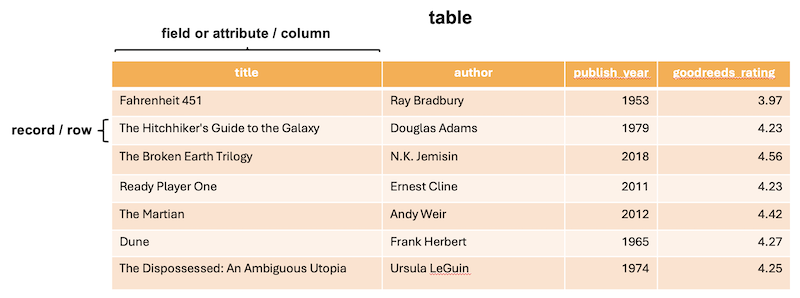
- table: A table is a collection of related data organized into rows and columns
- record: Each row in a table
- field or attribute: Each column in a table
- schema: the logical structure or design that defines how data is organized and stored in the database
Think of this last term, “schema”, as a blueprint outlining the relationships between tables and the data within them. There are lots of flow chart systems for organizing databases in order to indicate relationships between the data tables, what data and methods are included, and so on. Like with a camera, the best one is the one you’ll use.
Technically a database can have just one table, but just like with functions in Python, it’s often clearer and easier to maintain if each table has one purpose. We can then build relationships between the tables as we discussed.
Structured Query Language
Information is accessed and modified in a relational database using Structured Query Language (SQL).
SQL is a declarative language, rather than a procedural language like Python. In Python we have to write code that tells the computer exactly what we want it to do (we give directions). In SQL we tell the database what we want from it and the database figures out how to give us the information we want (we ask questions).
SQL is used to ASK QUESTIONS:
You can use SQL to ask questions (“to query”) about the data and it will respond by SELECTING any data relevant to the question.
For example, I might want to know “all students at IU who are Informatics majors”. Or get a list of “all juniors at SICE who are studying abroad in the Spring semester”.
SQL is used to EXECUTE A STATEMENT:
You can use SQL to make specific modifications to the database structure and to the data within. For example, SQL allows you to INSERT, UPDATE, MODIFY data or CREATE, DELETE, ALTER a data table.
Perhaps I need to UPDATE the record for an Informatics student named “Jackie Jackson” to show they have completed all core requirements.
Syntax
The convention in SQL is to CAPITALIZE any of the commands or keywords used, however the SQL will run just fine in lowercase too. (The more SQL you write, the less likely you are to want to type all caps…)
SHOW TABLES;
show tables;
In our examples in your book, we will make use of this CAPITALIZATION convention to help you better understand how SQL queries are constructed. If we need to indicate a variable, something you will fill in, we’ll borrow from the convention used in Flask routes, and use pointy brackets <variable>:
DESC <tablename>;
Finally, notice that all SQL commands typed in on a command line end with a semicolon ; and one common mistake when starting out with SQL, just like in CSS and JS actually, is to forget that semicolon. SQL statements can also be written on multiple lines to make them easier to parse with our eyes. As long as that semicolon is at the end, the new lines are ignored when the statement is executed.
If the cursor hangs after you hit Return when entering a SQL command, it may just be waiting for you to type in a semicolon!
Create a table
CREATE TABLE <tablename> (
  <attribute1name> datatype(size) [constraints],
  <attribute2name> datatype(size) [constraints],
  <attribute3name> datatype(size) [constraints]
) ENGINE=INNODB;
- Commas are used to separate attributes, but not end a list of them
ENGINE=INNOBis enforces referential integrity, basically it’s there to help us- Attribute names (column names), like variables, are case-sensitive. “FirstName”, for example, is NOT the same as “firstname”.
- Datatypes are required by SQL, note that some may also need a size indicated
- Constraints are optional, but often useful
Setting Datatypes
Each attribute (column) in a data table requires not only a name, but also a type for the data. Some choices are more common than others; we’ve listed ones you may encounter in your project.
Datatypes that store character or text data (such as names):
VARCHAR(maxsize)
Variable length character data with a maximum size of “maxsize” characters. Used when we don’t know how long the data is i.e. for first_name, title of a book, phone numbers because these often include non-numeric characters, etc.. this is a very commonly used datatype.
-- Erika Lee, Alexander Hayes, Michal Gordon
-- +1 812-855-6789
first_name VARCHAR(30)
phone VARCHAR(15)
email VARCHAR(50)
The length is up to you, but you want it to be long enough to cover the longest possible possibility for that data. So it’s okay to go a little longer than what you think you might need.
CHAR(fixedsize)
Fixed-length character data of size “fixedsize” characters. Used when we know exactly how long the data is.
-- IN, WI, NV, MD, etc..
state_abbr CHAR(2)
Datatypes that store larger amounts of character or text data:
TINYTEXT
Holds up to 255 characters. Good for text / character data that is several sentences long, like a short description of a book or a short social media post.
-- "I need to buy new window blinds, but I hate dealing with shady salespeople."
social_post TINYTEXT
TEXT
Holds a string of text up to 65,535 characters in length. Good for things like short books or chapters, memos, emails, longer posts, articles, etc…
-- "Unix-like Environments (sometimes written “*nix environments”) refer to ..."
chapter TEXT
Datatypes we use to store numeric data (such as price or quantity):
INT or INTEGER(size) and also FLOAT
Allocates 4 bytes to store a whole number if no size is specified (-2147483648 to 2147483647 for signed numbers, 0 to 4294967295 if unsigned). If specified, “size” is the number of digits.
-- 19, 1000000000, 6.5
age INT,
population INTEGER(10),
shoe_size FLOAT
DEC or DECIMAL(precision, scale)
Allocates precision number of digits with scale decimal places.
- Decimal(5,3) = ± 99.999
- Decimal(7,2) = ± 99,999.99
-- 873.54
price DEC(10,2)
Datatypes to store time and date data:
-- '2024-07-04', '19:30:00', '2024-07-04 19:30:00', '2024'
current_date DATE,
current_time TIME,
current_timestamp DATETIME,
current_year YEAR
DATE
Stores year, month, day in ‘YYYY-MM-DD’ format.
TIME
Stores hour, minute, second in ‘HH:MM:SS’ format.
DATETIME
Stores year, month, day, hour, minute, and second. Uses ‘YYYY-MM-DD HH:MM:SS’ format
YEAR
Stores the year as 4 digits.
We can also add optional constraints to our attributes:
CREATE TABLE students (
    id INT AUTO_INCREMENT PRIMARY KEY,
    name VARCHAR(50) NOT NULL
);
NOT NULL
Indicates that this attribute cannot have a null (empty) value. Any data inserted into this table must have a specified value for this attribute. Can be used for any attribute.
AUTO_INCREMENT
Used with an INT or INTEGER attribute. Automatically increments the value in the field each time a new record is added. Only one column in a table may be marked with this constraint. Used primarily for ID attributes.
PRIMARY KEY
This unique, not null (not empty) value is how we identify each unique record in our data. It is often an integer, because that makes indexing simple, but doesn’t have to be. The first column in each table will be a primary key. (In i211, we will make these integers.)
Remember, this ability to set a primary key for each record in a table is a step up from using part of the record as the identifier. (What if we are identifying people by name and we had two Alexander Hayes?? 😱) How do we know for sure we are interacting with the right person? A unique ID helps solve that problem.
Create a books table
Let’s write the SQL to create a table called books to hold data with the following types:
- unique
idnumber used as the primary key (and auto incremented) - required
title(up to 255 characters) - required
author(up to 100 characters) publish_yearthat holds a yeargoodreads_ratingstored as a decimal number with 3 digits and 2 decimal places
CREATE TABLE books (
    id INT AUTO_INCREMENT PRIMARY KEY,
    title VARCHAR(255) NOT NULL,
    author VARCHAR(100) NOT NULL,
    publish_year YEAR,
    goodreads_rating DECIMAL(3,2)
);
Getting Information About a Database
SQL lets us check our how many data tables we have:
SHOW TABLES;
We can also see what attributes (columns) a table contains:
DESC <tablename>;
What this interaction looks like:
MariaDB [i211u24_ebigalee]> CREATE TABLE books (
    ->     id INT AUTO_INCREMENT PRIMARY KEY,
    ->     title VARCHAR(255) NOT NULL,
    ->     author VARCHAR(100) NOT NULL,
    ->     publish_year YEAR,
    ->     goodreads_rating DECIMAL(3,2)
    -> );
Query OK, 0 rows affected (0.033 sec)

MariaDB [i211u24_ebigalee]> SHOW TABLES;
+----------------------------+
| Tables_in_i211u24_ebigalee |
+----------------------------+
| books                      |
+----------------------------+
1 row in set (0.001 sec)

MariaDB [i211u24_ebigalee]> DESC books;
+------------------+--------------+------+-----+---------+----------------+
| Field            | Type         | Null | Key | Default | Extra          |
+------------------+--------------+------+-----+---------+----------------+
| id               | int(11)      | NO   | PRI | NULL    | auto_increment |
| title            | varchar(255) | NO   |     | NULL    |                |
| author           | varchar(100) | NO   |     | NULL    |                |
| publish_year     | year(4)      | YES  |     | NULL    |                |
| goodreads_rating | decimal(3,2) | YES  |     | NULL    |                |
+------------------+--------------+------+-----+---------+----------------+
5 rows in set (0.001 sec)
Modifying a table
Right now, we have a table set up, but no data within the table. To add data, and otherwise manage that information, we need SQL to execute statements that modify the table.
NOTE: Once we run a query to make changes in SQL the changes are PERMANENT until you run a query to change things again. You do not need to “save” anything before you log out.
Drop a table
It’s possible to delete a table. If our table has data inside, that data will be deleted as well. Feel free to drop and re-add the books table for practice.
DROP TABLE <tablename>;
Alter a table
We can also make changes to the structure of our tables without necessarily dropping them.
If we forgot an attribute entirely, we can fix that by adding a new attribute:
ALTER TABLE <tablename> ADD <attributename> <datatype> <constraints>;
<tablename>is the table’s name<attributename>is the name of the attribute we want to change<datatype>is the new datatype we want for<attributename><constraints>are any optional constraints we want<attributename>to have
Let’s ALTER our books table to include an attribute for a genre. “COLUMN” is optional here. Run the following commands and after each, use DESC books; to see the alterations.
ALTER TABLE books
ADD COLUMN genre VARCHAR(50);
What if we had added an ISBN and made it the wrong datatype? We can ADD it:
ALTER TABLE books
ADD COLUMN isbn TINYTEXT;
If we messed up and gave the wrong datatype to one of our attributes, we can fix that using MODIFY:
ALTER TABLE books
MODIFY COLUMN isbn INT;
We can also drop/delete an attribute completely using DROP. Let’s go ahead and DROP the columns “genre” and “isbn” for now.
ALTER TABLE books DROP COLUMN genre;
ALTER TABLE books DROP COLUMN isbn;
Putting the data into data tables
Now that our structure is set up, we can use SQL to INSERT, UPDATE, SELECT or DELETE the data within:
INSERT INTO
To add data to any table, we’ll make use of INSERT:
INSERT INTO <tablename> (<attributes>,) VALUES (<values>)[,()] ;
<tablename>is the table’s name<attributes>are the column or attribute names separated by commas<values>are the values for those attribute names in the order they appear
When listing values, use single or double quotes around everything except numbers.
INSERT INTO books (title, author, publish_year, goodreads_rating)
VALUES ('Fahrenheit 451', 'Ray Bradbury', 1953, 3.97);
We can also add multiple lines of data at once:
INSERT INTO books (title, author, publish_year, goodreads_rating)
VALUES ('Dune', 'Frank Herbert', 1965, 4.27),
       ('The Dispossessed: An Ambiguous Utopia', 'Ursula LeGuin', 1974, 4.25);
INSERT the rest of the data into books either line by line or in multiple lines. When working with MariaDB on the command line, it can be useful to type in the SQL into a blank file, for example books.sql, and then copying and pasting at the prompt to run. It’s easy to make mistakes with commands this long.
'The Hitchhiker's Guide to the Galaxy', 'Douglas Adams', 1979, 4.23
'The Broken Earth Trilogy', 'N.K. Jemisin', 2018, 4.56
'Ready Player One', 'Ernest Cline', 2011, 4.23
'The Martian', 'Andy Weir', 2012, 4.42
With a little pattern matching, this can make adding data fairly straightforward.
Solution
  INSERT INTO books (title, author, publish_year, goodreads_rating)
  VALUES
  ('The Hitchhiker''s Guide to the Galaxy', 'Douglas Adams', 1979, 4.23),
  ('The Broken Earth Trilogy', 'N.K. Jemisin', 2018, 4.56),
  ('Ready Player One', 'Ernest Cline', 2011, 4.23),
  ('The Martian', 'Andy Weir', 2012, 2.32);
UPDATE
We can update data in any table in the relational database using the query “UPDATE … SET … WHERE …;”
UPDATE table
SET <attribute>  =  <newvalue>
[WHERE conditions] ;
The rating for 🛸 The Martian is too low. Let’s UPDATE that rating to “4.42”:
UPDATE books
SET goodreads_rating = 4.42
WHERE title = 'The Martian';
Without the WHERE to add the condition saying to update the rating only for a single title, we would have updated all ratings to be “4.42”. The WHERE narrows where the UPDATE is SET.
SELECT
SQL can also be used to ask questions of the data. We can select all of the data within the table. The basic SELECT query has 3 components to it:
SELECT <attributes we want to return/display separated by commas>
FROM <what table we will be querying>
WHERE <propositional logic conditionals that determine what gets displayed>
We can select all of the data if we want to, using * as a wildcard meaning “all”:
SELECT * FROM books;
The WHERE clause is optional. If omitted, the query will show ALL of the selected attributes from the table.
This means setting WHERE allows us to filter the data coming in from our SELECT. Being more precise with your query is especially useful when working with large datasets. We might want all of the data if we have 10 records, but what if we have 100000000? Returning a lot of records quickly can become slow, or at least not be all that helpful.
What if we just need to know something in particular about the data? Like who the author is for the book “Ready Player One”?
SELECT author
FROM books
WHERE title LIKE 'Ready Player One';
We can use % as a wildcard character to say things like “Select the author for the book where the title INCLUDES the word ‘Earth’”:
SELECT author
FROM books
WHERE title LIKE '%Earth%';
And because SQL understands that data set to be integers or dates can have math applied, we can ask questions like “Which of these books were written after the year 2000?”:
SELECT title
FROM books
WHERE publish_year > 2000;
Or “Which titles have a rating that’s less than 4.0?”
SELECT title
FROM books
WHERE goodreads_rating < 4.0;
Any math comparison will work on dates and numbers, including <= and >= and =.
We can even select both the “title” and “author” from a range of dates, using BETWEEN which also makes use of ‘AND’:
SELECT title, author
FROM books
WHERE publish_year BETWEEN 1950 AND 2000;
Other logical operators:
ORwill return true if either of the two conditions surrounding it is trueNOTwill return true if the condition is false, allowing us to use what we don’t want to select what we do
SELECT * FROM books
WHERE goodreads_rating = 4.25 OR goodreads_rating = 4.27;
SELECT * FROM books
WHERE NOT (title = 'The Martian');
We can also adjust how the information is returned and sort it as ASC ascending or DESC descending.
This is especially helpful for numeric data, and may or may not be what you expect alphabetically because the sorting is done by ASCII code. That means upper- and lowercase letters have different codes and the result may not be what you expect.
Run some examples similar to these to see what we mean:
SELECT title
FROM books
ORDER BY goodreads_ranking ASC;
SELECT author
FROM books
ORDER BY author DESC;
DELETE
And finally, we can delete a row of data from a table using the “DELETE FROM … WHERE …;” statement.
DELETE FROM table [WHERE conditions];
To DELETE the record for the title “Ready Player One”:
DELETE FROM books
WHERE title = 'Ready Player One';
Be careful with this. If your query isn’t written as you expect, you might end up deleting data you weren’t ready to delete. Best to select first and make sure you have the conditions right.
Summary
- We now have the ability to connect to a relational database
- The first step to a good database is to understand the data we want to structure and make a plan for how the tables and the data in them will interact - this skill is a focus for other courses
- Data tables can be CREATE(d) with attributes (with specified datatypes), or we might want to DELETE or ALTER
- Structured Query Language (SQL) also helps us INSERT, UPDATE or MODIFY data in data tables
- SQL is really great at asking questions of data so we can make specific SELECT(ions)
What we need next is an upgrade to our process such that SQL can be used to interact with a database FROM WITHIN our Flask application. We’ll do this using a Python library called PyMySQL.
Want more practice with SQL?
Footnotes
E. F. Codd. 1970. A relational model of data for large shared data banks. Commun. ACM 13, 6 (June 1970), 377–387. https://doi.org/10.1145/362384.362685
Peter Pin-Shan Chen. 1976. The entity-relationship model—toward a unified view of data. ACM Trans. Database Syst. 1, 1 (March 1976), 9–36. https://doi.org/10.1145/320434.320440
We use the phrase “fully normalized” intentionally here, as the version of normalization described by Codd in 1970 is what we now refer to as “First normal form” (or 1NF). The existence of the phrase “first normal form” implies the existence of 2nd, 3rd, 4th, and many other normal forms. These are of theoretical and some practical interest, but we do not want to spend much time on this point. On first glance: people often assume that goals like “remove redundancy” are critical, but in practice: some redundancy often exists for performance reasons. The theoretical guarantees of normal forms are helpful, but in practice: it means actual database systems have to chase foreign keys and spend more time “figuring out” where data is actually stored. “Denormalization” is therefore a trick to squeeze better performance out of systems.